Week 8: Selecting and Revalidating Operating Conditions
Product specifications and revalidation of an optimum
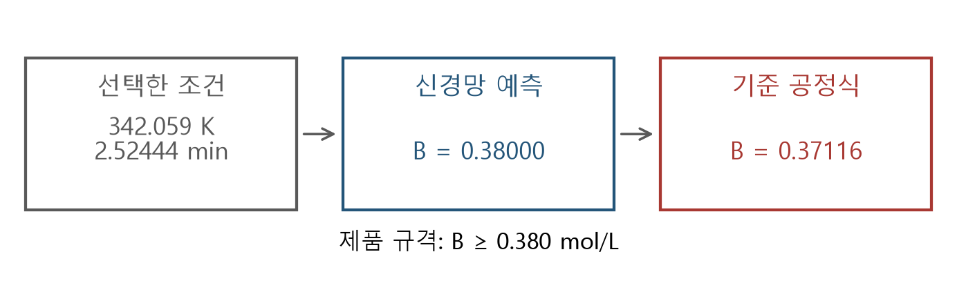
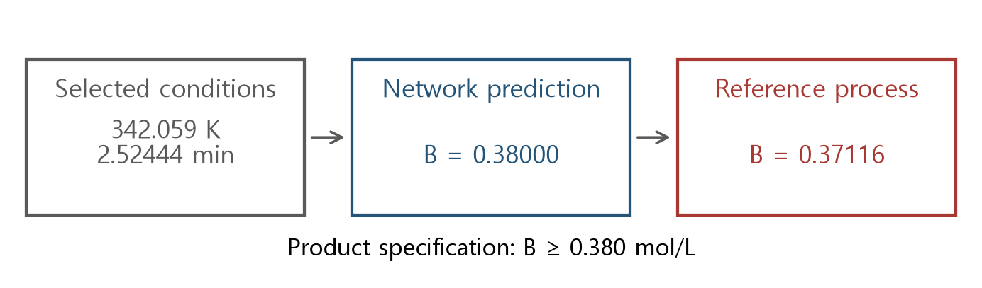
The optimized product concentration meets the specification of 0.380 mol/L. Yet the process equations give 0.371 mol/L at the same conditions. Should this candidate be accepted?
Revalidate the selected conditions, choose an acceptable candidate, and identify the next useful data.
Prediction validation and decision validation
Average error on independent evaluation data summarizes predictive quality across an input region. Optimization selects a few points with low cost, often near constraint boundaries.
Recompute product specifications, physical consistency, and cost at those decisions. Separately check whether the solver correctly represented the fitted model.
This week: these distinctions with the unchanged frozen network from Week 6.
Learning objectives and final report
- Prediction error, formulation error, and process constraint violation
- Cost comparison among candidates feasible in the reference process model
- Revalidation after margins and local data correction
- Reproducible records of models, data, solvers, and candidate selection
Final report: accepted candidate, rejection reasons, remaining checks, and additional data locations.
Reactor assumptions and variables
Reference process: ideal steady-state isothermal CSTR; consecutive first-order reactions A → B → C. Feed concentrations: A 1.2 mol/L, B and C zero. Constant density and flow.
Temperature T spans 310-350 K and residence time τ spans 2-10 min. At fixed F = 1 L/min, V = Fτ, so τ is also a reactor-sizing decision.
Changing τ in an existing fixed-size vessel requires changing flow or another condition. That requires a revised cost and process formulation.
Temperature-dependent reaction rates
Rate constants have units min⁻¹, activation energies are J/mol, and R = 8.314 J/(mol·K). At 330 K, k₁ = 0.2 and k₂ = 0.1.
Temperature is externally maintained; this model includes no energy balance or cooling-capacity limit.
Unlike the 6000 K and 5000 K sensitivities in Weeks 1–4, this reference uses E/R=40000/8.314 and 50000/8.314 K. Rates agree at 330 K but differ elsewhere. Revalidate the Week 6 weights with the reference used in Weeks 6–8.
Reference process equations and product specifications
Specifications are ≥ 0.38 and ≤ 0.25 mol/L. Concentrations must be nonnegative and sum to 1.2 mol/L.
Revalidation with these equations is conditional on their assumptions. Actual equipment requires additional checks on dynamics, heat management, measurement error, and other operating limits.
Calculate A first, then balance B formation against its outflow and onward reaction. C follows from formation out of B. Use this sequence at the identical T,τ when comparing the network with the reference process.
Cost criterion and comparison baseline
J is measured in $/h. Assume a volume cost of 12 $/(L·h) and, at fixed flow, a heating coefficient of 0.24 $/(K·h). With F = 1, the volume term becomes 12τ.
This cost compares designs meeting product specifications. It includes neither sales revenue nor actual equipment quotations.
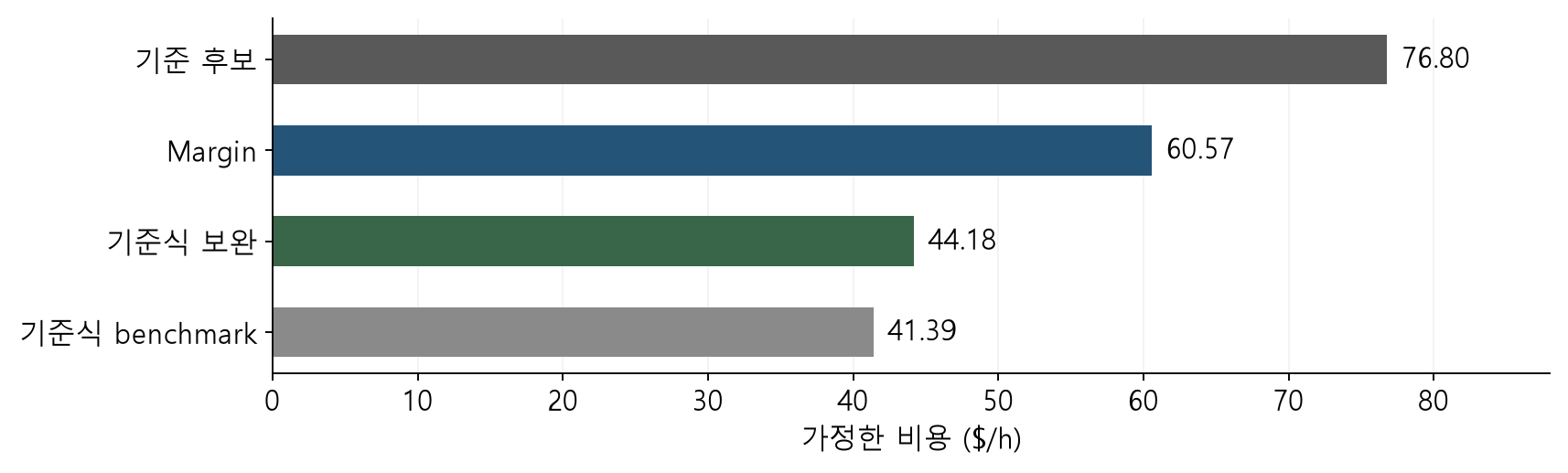
Baseline: T = 330 K, τ = 6 min; cost 76.80 $/h.
At flow 1 L/min, τ=6 min means volume 6 L. Volume cost is 12×6=72 $/h and temperature cost is 0.24×(330−310)=4.8 $/h, totaling 76.8 $/h. This baseline is checked for specifications as well as cost.
The surrogate optimization problem
Input bounds and scaling match Week 6. The objective is twelve times the Week 6 cost index, so the unadjusted model has the same optimal input.
Use the ReLU MILP from Weeks 5 and 6. The Week 7 cost-epigraph LP does not automatically apply to concentration constraints.
Multiplying every objective value by positive 12 preserves ranking, so the optimal input matches Week 6 while the cost unit changes. Specifications are imposed on network predictions; that ranking alone does not establish feasible costs for the reference process.
Separating errors from termination status
| Check | Quantities compared |
|---|---|
| Formulation error | MILP output and network forward output at the same input |
| Prediction error | Network output and reference process output |
| Constraint violation | Reference output and product specifications |
| Optimization gap | Incumbent and valid bound for the fitted model |
The unadjusted solve has MILP/forward disagreement below 10⁻¹² mol/L. Its reference product concentration still misses the specification.
Average prediction error and decision-point error
Generate 997 inputs uniformly over the full box, separately from training. RMSE is 0.00535 for A, 0.00439 for B, and 0.00527 for C, in mol/L.
At the optimized candidate, B is overpredicted by 0.00884 mol/L. Since its prediction lies exactly on the specification boundary, this error causes a violation.
Report error at the optimized candidate alongside independent average error so that specification violations at the selected point are visible.
Optimization can reduce cost by reducing specification slack until predicted B touches its lower bound. At that point even a small overprediction causes violation. Evaluate the selected point’s error direction and slack separately from domain-average RMSE.
Reference revalidation of the unadjusted candidate
| Quantity | Value |
|---|---|
| T / τ | 342.0593 K / 2.52444 min |
| Predicted B / reference B | 0.380000 / 0.371157 mol/L |
| Reference C | 0.178136 mol/L |
| B shortfall | 0.008843 mol/L |
| Calculated cost | 37.9875 $/h |
Reject this candidate because it violates the product specification. Its lower cost does not make it an improvement over a feasible baseline.
Predicted B slack is zero and overprediction is 0.008843, so reference slack is −0.008843. C retains slack 0.25−0.178136=0.071864 mol/L. Failure of even one required specification rejects the candidate.
Input domain and data support
A candidate inside the training box can still have large error if nearby data are sparse or the response varies rapidly. Being inside the box alone does not guarantee accurate interpolation.
Inspect input ranges, scaled coordinates, distances to nearby training points, and errors near boundaries. An expanded optimization domain needs separate model validation.
Recompute valid formulation bounds for the new domain as well.
Physical consistency and product feasibility
Record the concentration sum, negative concentrations, and product specifications separately. An exact sum can coexist with low B; positive concentrations can coexist with excessive C.
The Week 4 equality projection enforces its specified linear equality. It does not guarantee product specifications or accurate nonlinear process responses.
Margins from one-sided errors
Overprediction of B and underprediction of C are the adverse directions. A separate calibration grid gives = 0.02130 and = 0.01305 mol/L.
These are maxima observed at 961 points, not proven bounds over the continuous domain. Reevaluate the new candidate with the process equations.
B has a lower requirement, so guard against the model predicting too much. C has an upper limit, so guard against predicting too little. Opposite inequality directions explain why one margin is added and the other subtracted.
Calculating one-sided margins
Define e=prediction−reference. Positive e is adverse for B; negative e is adverse for C.
| Quantity | B lower limit | C upper limit |
|---|---|---|
| Original specification | Reference B≥0.38 | Reference C≤0.25 |
| Applied margin | δ_B=0.02130 | δ_C=0.01305 |
| Required prediction | B̂≥0.40130 | Ĉ≤0.23695 |
| At the assumed error limit | 0.40130−0.02130=0.38 | 0.23695+0.01305=0.25 |
The last row applies when the error limit holds at that input. The maximum over 961 calibration points does not prove a bound at every unseen point. Reevaluate the next candidate with the reference process even after adding margins.
Sample margins are δ_B=max(0,maxᵢ e_B,i) and δ_C=max(0,maxᵢ(−e_C,i)). B errors [−0.003,0.008,0.002] give 0.008; C errors [0.004,−0.006,−0.001] give 0.006. Unlike an absolute-error maximum, these select only the direction that can violate the specification.
Cost and specifications of the margin candidate
| Quantity | Result |
|---|---|
| T / τ | 329.1148 K / 4.66529 min |
| Reference B / C | 0.392935 / 0.174547 mol/L |
| Reference feasibility | Specifications met |
| Cost | 60.5710 $/h |
| Savings versus baseline | 16.2290 $/h |
Using a large error observed anywhere in the domain as a margin can be costly in some regions. Compare the margin with error at the actual selected point.
Savings from the baseline are 76.8000−60.5710=16.2290 $/h. First confirm positive reference slacks: 0.012935 for B and 0.075453 mol/L for C; then report the savings.
Choosing additional data locations
Form a 3 × 3 grid around the unadjusted candidate using offsets −0.06, 0, +0.06 on each scaled axis. Clip to the original input box and obtain nine reference outputs.
Local residual correction: these data, separate from the 997 final-evaluation inputs
Choose points to examine constraint boundaries, the current candidate, and error direction. For physical experiments, include accessible conditions and experimental costs.
A local residual model and restricted domain
Fit an affine model to reference-minus-prediction residuals at the nine points. Restrict optimization to their bounding box and apply a 0.002 mol/L margin to both product constraints.
This margin is heuristic. Affine correction preserves the MILP structure but provides no uniform bound on residual error.
The correction target is reference minus prediction. At a point overpredicting B by 0.008843, the desired correction is −0.008843. Reversing the sign would raise an already inflated prediction; check corrected output explicitly at one point.
Local-data coordinates and the regression matrix
Candidate (342.0593 K,2.52444 min) has scaled coordinates [(342.0593−310)/40,(2.52444−2)/8]≈[0.80148,0.06556].
| Axis | Scaled offset | Physical offset |
|---|---|---|
| Temperature | ±0.06 | ±2.4 K |
| Residence time | ±0.06 | ±0.48 min |
design = np.column_stack((np.ones(len(x_local)), x_local))
residual = reference_y - network_y
beta = np.linalg.lstsq(design, residual, rcond=None)[0]
corrected_y = network_y + design @ beta
For nine inputs, design is (9,3), the three-component residual is (9,3), and beta is (3,3). Multiplying a row [1,x₁,x₂] by beta gives three corrections. Restrict the next optimization to the fitted region and check remaining error at the new candidate.
Substituting the fitted correction coefficients
The recorded B correction coefficients are [−0.0160962605,0.0074357617,0.0823403944]. At local candidate (339.815193 K,2.870934 min), x₁=0.745379824 and x₂=0.108866748.
| B correction term | Value [mol/L] |
|---|---|
| Intercept | −0.0160962605 |
| Temperature-coordinate term | 0.0074357617×0.745379824=0.0055424667 |
| Residence-time-coordinate term | 0.0823403944×0.108866748=0.0089641309 |
| Sum | −0.0015896628 |
Adding this to the original network prediction B≈0.3835896628 gives corrected prediction 0.382000. The reference value at the same input is 0.3768201356, leaving error 0.0051798644.
Least squares reduces the summed squared errors of nine points. It does not require interpolation of every point or exact prediction at a new candidate. Correctly computed regression coefficients still require candidate revalidation.
Failed revalidation after local correction
| Quantity | Result |
|---|---|
| T / τ | 339.8152 K / 2.87093 min |
| Corrected prediction B | 0.382000 mol/L |
| Reference B | 0.376820 mol/L |
| B shortfall | 0.003180 mol/L |
| Cost | 41.6069 $/h |
Reject this candidate despite nine new data points and a restricted local domain. Its corrected-model error exceeds the 0.002 margin.
The new residual at the candidate becomes useful follow-up data. Do not report the rejected candidate’s cost as achieved savings.
The corrected model predicts 0.382 while the reference gives 0.376820. Subtracting the reserved margin 0.002 from error 0.005180 leaves shortfall 0.003180. Adding data does not by itself establish that remaining error lies within the margin.
Repairing a candidate with the reference process equations
Because this reference model is inexpensive, fix T = 339.8152 K and directly calculate the smaller τ satisfying B = 0.382. Use the original input range, without the local-correction box restriction.
At τ = 3.08559 min, reference C is 0.199530 mol/L and cost is 44.1828 $/h. All original specifications are met.
Specification feasibility of this candidate is checked directly with the reference equations; it lies outside any guarantee supplied by the local correction model.
From the B specification to a quadratic in residence time
At fixed temperature, k₁ and k₂ are numbers. Set B to target b and multiply by the positive concentration denominator.
| Step | Relation |
|---|---|
| Set B=b | 1.2k₁τ=b(1+k₁τ)(1+k₂τ) |
| Expand denominator | 1.2k₁τ=b[1+(k₁+k₂)τ+k₁k₂τ²] |
| Collect terms | bk₁k₂τ²+[b(k₁+k₂)−1.2k₁]τ+b=0 |
At 330 K and b=0.4, this is 0.008τ²−0.12τ+0.4=0. Dividing by 0.008 gives (τ−5)(τ−10)=0. B≥0.4 holds between the roots, [5,10].
At fixed temperature, cost increases with τ, so check 5 min first. It gives C=0.1×5×0.4=0.2≤0.25. At 10 min, C=0.4 violates the cap; the B condition alone is insufficient.
Computing the smaller root and revalidating the candidate
At T=339.8152 K and b=0.382, calculate a=bk₁k₂ and d=b(k₁+k₂)−1.2k₁. A negative discriminant means there is no real residence time with B=b at this temperature.
k1 = 0.2 * np.exp(40000 / 8.314 * (1/330 - 1/T))
k2 = 0.1 * np.exp(50000 / 8.314 * (1/330 - 1/T))
a = b * k1 * k2
d = b * (k1 + k2) - 1.2 * k1
disc = d*d - 4*a*b
tau = 2*b / (-d + np.sqrt(disc))
Here k₁≈0.3047, k₂≈0.1693/min and τ≈3.08559 min. This smaller-root formula uses a>0,d<0,disc≥0. Check the original τ bounds and reference B,C for each candidate.
Reference C≈0.199530<0.25 and cost is 12×3.08559+0.24×(339.8152−310)≈44.1828 $/h. Savings from the original baseline are 76.8−44.1828=32.6172 $/h.
Rationalizing the smaller-root formula
For aτ²+dτ+b=0, define D=d²−4ab. With a>0,d<0,D≥0, the smaller root is (−d−√D)/(2a). Multiply numerator and denominator by −d+√D.
Since d²−D=4ab, cancellation gives the last expression. Replacing subtraction of similar positive values −d and √D with addition reduces loss of significant digits.
At 330 K,b=0.4, a=0.008,d=−0.12,D=0.0016 and √D=0.04. The smaller root is 0.8/(0.12+0.04)=5; the larger is (0.12+0.04)/0.016=10 min. Substitute roots back into the original B equation and C specification before accepting a candidate.
Reference-model optimization for comparison
At each T, solve the quadratic equation for the smaller τ giving B = 0.38. Check τ bounds and the C specification, then use 4,001 temperature grid points and a scalar search near the best grid point.
Comparison candidate: T = 344.9116 K, τ = 2.75110 min; cost 41.3920 $/h.
This supplies a feasible benchmark, not a certified global bound over the continuous domain. Report cost differences as observed benchmark differences.
At fixed temperature, cost increases with τ, so first inspect the smallest τ satisfying the B lower limit. Residence-time bounds and the C limit still apply. The smaller root at an arbitrary temperature is not automatically feasible.
Reference process results by candidate
| Candidate | B (mol/L) | Cost ($/h) | Specs |
|---|---|---|---|
| Baseline | 0.40909 | 76.800 | Met |
| Unadjusted MILP | 0.37116 | 37.988 | Violated |
| Margin MILP | 0.39293 | 60.571 | Met |
| Local correction | 0.37682 | 41.607 | Violated |
| Reference repair | 0.38200 | 44.183 | Met |
| Reference benchmark | 0.38000 | 41.392 | Met |
Every B value uses the same reference process equations. Specification checks include B, C, nonnegative concentrations, and the concentration sum.
Check each row using its complete reference composition. Although the table displays B, also evaluate C, the sum, and nonnegativity. A failed row’s low cost is excluded from rankings of feasible savings.
Cost comparison among feasible candidates
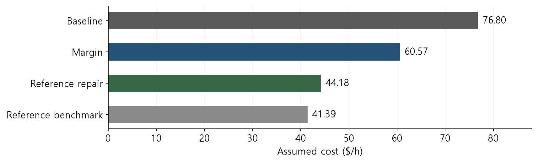
The reference-repaired candidate costs 32.6172 $/h less than the initial baseline, with an observed benchmark difference of 2.7908 $/h.
All values depend on the assumed cost coefficients. Record reference evaluations, model training, and optimization time separately.
Subtracting benchmark 41.3920 from repaired-candidate cost 44.1828 gives 2.7908 $/h. This compares two checked candidates. Without a proof that the benchmark is globally optimal, it is not certified regret relative to the global optimum.
Iteration procedure and acceptance criteria
- Fix the fitted model, domain, context, specifications, and cost.
- Obtain a candidate and check forward agreement and solver termination.
- Check original constraints with the reference equations. On failure, retain a feasible incumbent.
- Add data, revise the model or region, and revalidate the next candidate.
Convergence of trust-region methods requires conditions on model accuracy and acceptance rules. Those conditions have not been established for this local correction procedure, so convergence is not guaranteed.
Reproducibility items in the final report
| Category | Record |
|---|---|
| Model/data | Frozen-weight hash, scaling, training/calibration/evaluation/update data |
| Problem | Input bounds, fixed context, units, objective, and constraints |
| Computation | Solver/version/status/gap/time and forward error |
| Decision | Reference output, violations, cost, and acceptance by candidate |
| Remaining checks | Reference assumptions, dynamics, heat management, and experiments |
Running the lab and report assignment
python -m pip install -r requirements.txt
python week08_lab.py --output-dir my-results
The bundle includes the frozen Week 6 network and required calculation functions. It saves a results JSON, candidate-comparison CSV, independent evaluation data, and nine update points.
Change a margin or local-grid width once, then revalidate the new candidate against the original specifications. Record data count and cost and explain acceptance or rejection.