Week 6: Solve Time and Results in Neural-Network Optimization
Reactor conditions that meet product specifications
A reactor design review requires repeated searches over temperature and residence time. After finding conditions that meet the product specifications, we still need to assess how much improvement may remain.
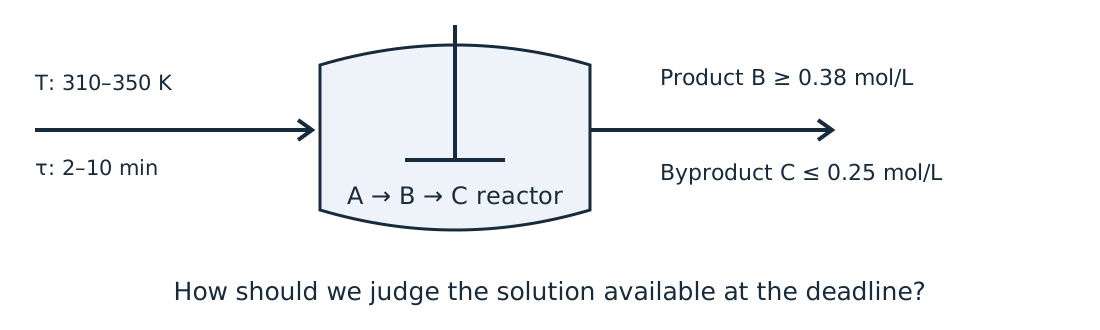
This week: unfinished-solve assessment, bounds, and formulation choices.
The problem and the comparison conditions
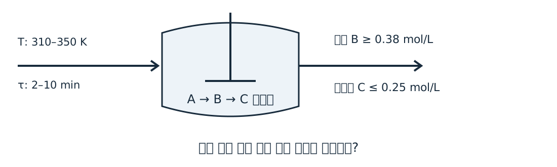
Add temperature as an input to the Week 5 reactor setting. At a fixed flow of 1 L/min, residence time also selects reactor volume and is therefore a design variable.
Hold the fitted ReLU model, input domain, objective, and product specifications fixed while comparing formulations. Arbitrarily shrinking the temperature interval changes the design problem.
Solver for all LPs and MILPs: open-source HiGHS.
Learning objectives for formulations and solver results
- Incumbent objective, objective bound, and gap
- Interval propagation versus LP-based bound tightening
- Frozen network and scaling in Pyomo and OMLT
- Termination, time, forward agreement, and constraint residuals
Review the Week 5 Big-M equivalence and input-bound calculations first.
The frozen network and its MILP representation
For a ReLU input a with valid bounds L ≤ a ≤ U and L < 0 < U, use these inequalities with binary z.
Weights, biases, and scaling remain fixed. The full problem is an MILP when the other constraints and objective are linear. Exact network representation is separate from process prediction error.
Incumbents, objective bounds, and gaps
For minimization, the incumbent is the best integer-feasible solution found so far. Its objective value supplies an upper bound that, together with a valid lower bound, brackets the optimum.
An upper bound of 100 and lower bound of 80 give an absolute gap of 20 and a relative gap of 20% under this definition. Without an incumbent this gap is unavailable; near a zero objective, also report the absolute gap.
A feasible design supplies an upper bound because there is no need to select anything more expensive. A relaxation admits even more favorable choices and supplies a lower bound. The interval between them is the remaining possible improvement.
How branch-and-bound progresses
Relaxing binaries to continuous intervals gives an LP lower bound for minimization. A fractional binary can be branched into subproblems with z = 0 and z = 1.
An integer-feasible solution updates the incumbent. Infeasible nodes and nodes whose lower bounds cannot improve the incumbent need no further search.
Valid bounds from open nodes form the global lower bound. HiGHS also uses presolve, cuts, and heuristics, so the original LP relaxation value can differ from the final solver bound.
If the incumbent costs 100 and a node has lower bound 105, every integer solution in that node costs at least 105, so it can be pruned. A node bounded by 80 may still contain an improvement below 100 and needs further investigation.
The continuous relaxation of a ReLU
Relaxing z to [0, 1] and eliminating it gives this triangle for L < 0 < U.
At a = 0, the largest allowed h is −UL/(U − L). It is 0.5 when L = −1 and U = 1, although the ReLU output is zero.
This triangle is the convex hull of the scalar (a, h) graph. Correlations across inputs and neurons may require additional constraints.
With L=−1,U=1 and a=0, the upper bound is (0+1)/2=0.5. Allowing this value above the true h=0 creates relaxation slack. Tighter valid bounds can reduce it.
Two neurons coupled by an equality
Dimensionless example: a dependence missed by box bounds
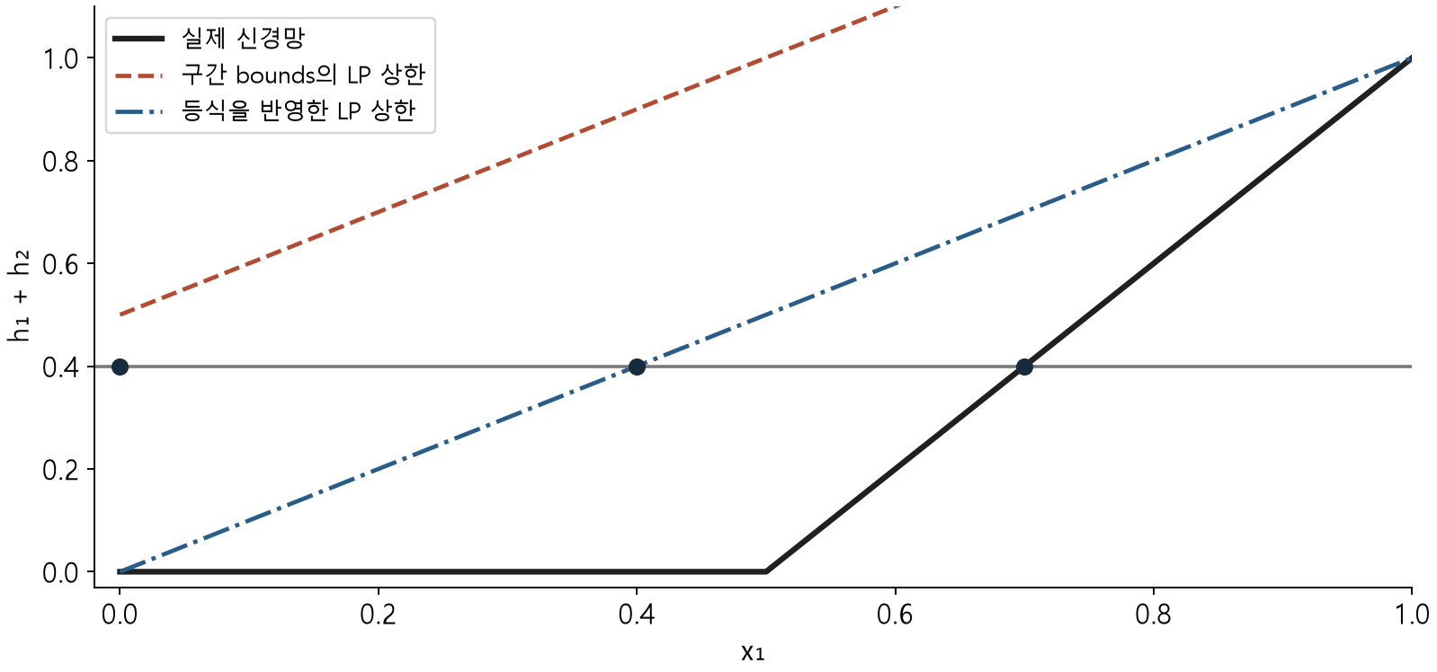
Using only the input box gives [−1, 1] for both pre-activations. The input equality, however, makes the first pre-activation identically zero.
Box bounds alone allow combinations x₁=x₂=0 or 1. The equality x₁+x₂=1 excludes them and fixes the first pre-activation at zero. Individual variable ranges and relations between variables therefore contain different information.
The exact solution of the two-neuron example
The minimum is therefore 0.7. The MILP with box bounds and the MILP using the equality both attain this optimum.
The LP relaxation can place h above the network output, so this conclusion does not immediately apply to its solution.
When x₁≤0.5, the second ReLU is also zero and cannot meet 0.4. In its active branch, solve 2x₁−1≥0.4 to get x₁≥0.7. Substituting 0.7 verifies feasibility and makes the lower limit attainable.
LP relaxations before and after tightening
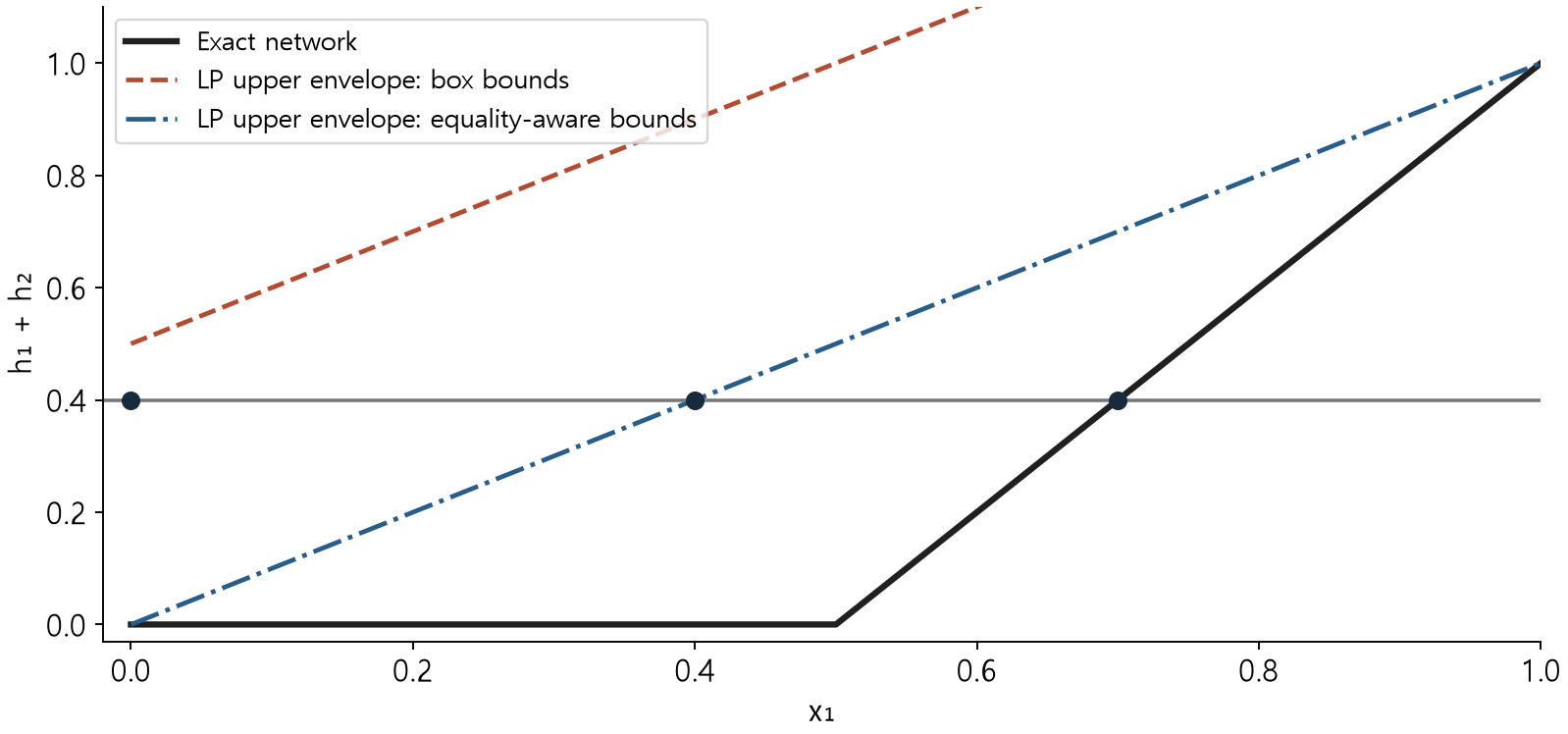
The original LP allows = 0.4 even at = 0. Enforcing = 0 raises the LP optimum to 0.4, still below the MILP optimum of 0.7.
Relaxed solutions versus the actual network
Each formulation minimizes x₁ with x₂=1−x₁ and required output sum 0.4.
| Formulation | x₁,x₂ | Allowed h₁,h₂ | Actual ReLU output | Interpretation |
|---|---|---|---|---|
| Box-bound LP | 0,1 | 0.4,0 | 0,0 | Inflated h₁ meets the limit |
| Equality-aware LP | 0.4,0.6 | 0,0.4 | 0,0 | Inflated h₂ meets the limit |
| MILP | 0.7,0.3 | 0,0.4 | 0,0.4 | Matches the original output |
After incorporating the equality, the second triangle has upper bound h₂≤x₁. Thus h₂≥0.4 requires x₁≥0.4. Yet at x₁=0.4, the actual a₂=−0.2 gives zero ReLU output. Improving the lower bound does not make the relaxation identical to the graph.
Branching and termination in the two-neuron example
After enforcing h₁=0, only h₂’s binary z₂ remains. Its bounds are L=−1,U=1 and a₂=2x₁−1. Adding the root LP rows h₂≤z₂ and h₂≤2x₁−z₂ gives h₂≤x₁. Since h₂≥0.4, x₁≥0.4 is a lower bound.
| Problem | Calculation | Conclusion |
|---|---|---|
| Root LP, 0≤z₂≤1 | x₁=0.4,h₂=0.4,z₂=0.4 is feasible | lower bound 0.4; not integer |
| Child z₂=0 | h₂=0 contradicts h₂≥0.4 | infeasible; close |
| Child z₂=1 | h₂=2x₁−1≥0.4 | minimum attained at x₁=0.7 |
The children cover both possible binary values. One is infeasible and the other has minimum 0.7, establishing a global lower bound of 0.7. It matches feasible cost 0.7, so the gap is zero.
With several open nodes, the smallest node lower bound identifies a branch that may still improve the incumbent. A branch whose bound reaches the incumbent cannot improve it and can be closed. A real solver may use different branching and cuts.
The domain over which bounds are valid
Bounds must hold at every allowed input. Training-sample extrema alone do not guarantee coverage of the full input domain.
Overly narrow bounds can cut off valid network points. Wider valid bounds preserve the integer graph but can weaken its relaxation.
Bounds computed using product specifications are valid only over that constrained feasible set. Recheck them when specifications or the input domain change.
Interval propagation with weight signs
Suppose the previous layer satisfies ℓ ≤ h ≤ u, with = max(w, 0) and = min(w, 0).
After a ReLU, pass [max(0, L), max(0, U)] to the next layer. This is inexpensive but does not check whether different variable extremes can occur simultaneously.
If h₁=h₂ but both are represented only by [0,1], interval arithmetic gives h₁−h₂ in [−1,1], although the true difference is zero. Interval propagation quickly constructs valid outward bounds but loses such dependencies.
LP-based bound tightening
Let P be an LP relaxation containing the network MILP feasible set. Minimize and maximize each pre-activation over P.
This is optimization-based bound tightening, or OBBT. The lab solves 54 LPs over the full input domain without product specifications, then rebuilds the MILP with the resulting bounds.
The lower-bound problem asks how small this neuron can become over every allowed input. The upper-bound problem maximizes the same expression. Solving over a relaxation containing every original network point produces bounds that do not exclude those points.
Suppose minimizing a stops with feasible value −0.2 and valid lower bound −0.6. Its true minimum lies in [−0.6,−0.2]. Use −0.6 as the neuron’s lower bound: using −0.2 could cut off a valid point with a=−0.4. For a maximum, use a valid upper bound instead.
Handling neurons with fixed activation states
These cases need no binary variable. Only neurons whose intervals cross zero remain candidates for branching.
Hand-built MILP binary counts: 24 with loose bounds, 22 with interval propagation, 19 with LP-OBBT. Counts before solver presolve.
Input scaling and physical units
Reuse exactly the offsets and scales used during fitting. Supplying physical-input bounds as scaled-input bounds changes the domain evaluated by the network.
Outputs in this lab already use mol/L. If outputs were standardized, include the fixed inverse transform before connecting product specifications.
330 K and 6 min are both interval midpoints, giving scaled input [0.5,0.5]. Swapping input order makes temperature weights read residence time. Comparing forward outputs at identical physical inputs also detects this ordering error.
Objective constants and relative gaps
Educational objective: residence time + temperature increase weighted by α. Unit: min-equivalent score.
Dropping the constant 2 preserves the optimizer but changes the denominator of a relative gap. The lab reports objectives and bounds with the constant included.
Computing gaps with an objective constant
Keep the same incumbent and valid bound, removing only constant 2 from the objective.
| Calculation | J with constant | J−2 without constant |
|---|---|---|
| Feasible objective | 3.2 | 1.2 |
| Valid lower bound | 2.8 | 0.8 |
| Absolute gap | 3.2−2.8=0.4 | 1.2−0.8=0.4 |
| Relative gap | 0.4/3.2=12.5% | 0.4/1.2≈33.3% |
Subtracting the same number from every candidate preserves ranking and the optimal input. The relative-gap denominator changes, however. Percentages alone cannot compare solve quality when the objective definitions differ.
Without an incumbent there is no value for that denominator. Report the valid bound and absence of a feasible solution; do not interpret initialized variables as the answer.
Roles of the open-source tools
| Tool | Role |
|---|---|
| NumPy | Network forward pass and optional refitting |
| Pyomo | Variables, objective, and process constraints |
| OMLT | Frozen-network constraints in Pyomo |
| HiGHS / highspy | LP and MILP solution |
All LPs and MILPs use open-source HiGHS under the MIT license.
Check the input ordering, scaling, and bounds of the constraints generated by OMLT. HiGHS official site
Connecting OMLT to process constraints
Build definition from the weights and scaling, then connect the process constraints. nn.inputs uses physical units; scaled_inputs holds transformed inputs.
model.nn = OmltBlock()
model.nn.build_formulation(ReluBigMFormulation(definition))
model.product = pyo.Constraint(expr=model.nn.outputs[1] >= .38)
model.byproduct = pyo.Constraint(expr=model.nn.outputs[2] <= .25)
model.obj = pyo.Objective(
    expr=model.nn.inputs[1] + .02*(model.nn.inputs[0]-310))
outputs[1] is B and outputs[2] is C. inputs[0] is temperature in K; inputs[1] is residence time in min. OMLT scaling equalities connect physical inputs to network coordinates; the objective must use the intended physical quantities.
Reproducing Week 5 with OMLT
First check the existing interpolant with residence time as its sole decision, at 330 K and a feed A concentration of 1.2 mol/L. Apply B ≥ 0.40 and C ≤ 0.25 mol/L.
| Formulation | Minimum residence time [min] | Generated binaries |
|---|---|---|
| Hand-built | 5.353846 | 3 |
| OMLT | 5.353846 | 4 |
This OMLT version creates a binary for each ReLU. The hand-built model represents one always-active neuron linearly, using one fewer binary while giving the same outputs.
Choosing temperature and residence time
Units: concentrations mol/L, temperature K, residence time min. Additional constraint: nonnegative predicted concentrations.
Architecture: two inputs, two hidden layers of 12 ReLUs each, and three linear outputs. All comparisons: the same frozen coefficients.
Fitting and independently evaluating the frozen model
Generate concentrations at 1,200 training inputs from ideal isothermal A → B → C CSTR balances and fit with 6,000 NumPy Adam updates. Evaluate physical-unit errors at 500 independent random inputs.
| Component | Test RMSE [mol/L] |
|---|---|
| A | 0.00546 |
| B | 0.00440 |
| C | 0.00564 |
The default lab loads the supplied coefficients. --refit optionally refits them; weights never change during optimization.
Comparing relaxation values across bounds
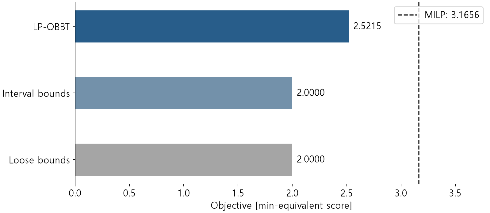
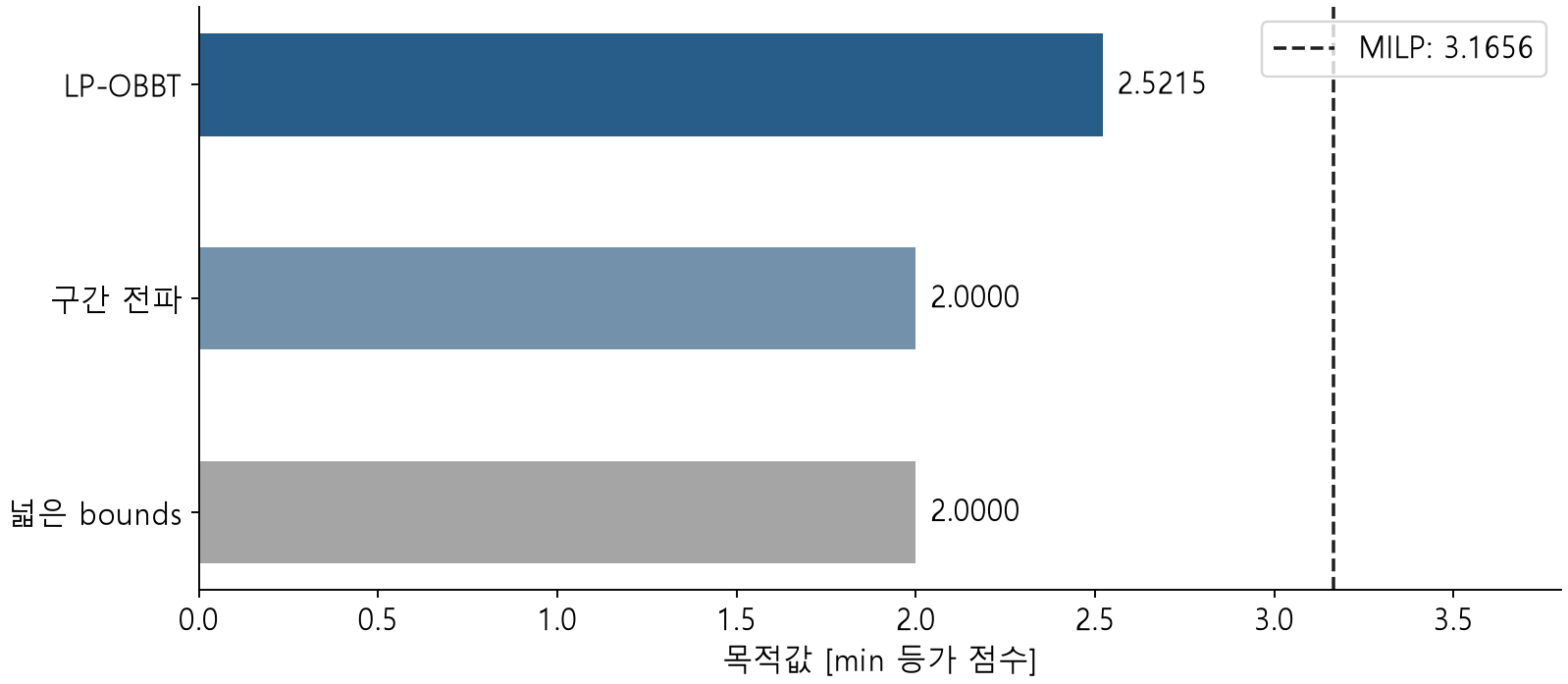
LP-OBBT raises the original LP lower bound from 2.0000 to 2.5215. All three MILPs attain 3.1656. All three comparisons use the same predictor.
The interval from lower bound 2.5215 to feasible value 3.1656 is about 0.6441, narrower than 1.1656 from the loose bound 2.0000. Predictions are unchanged, but less optimality uncertainty remains at the start of the search.
Timing including bound computation
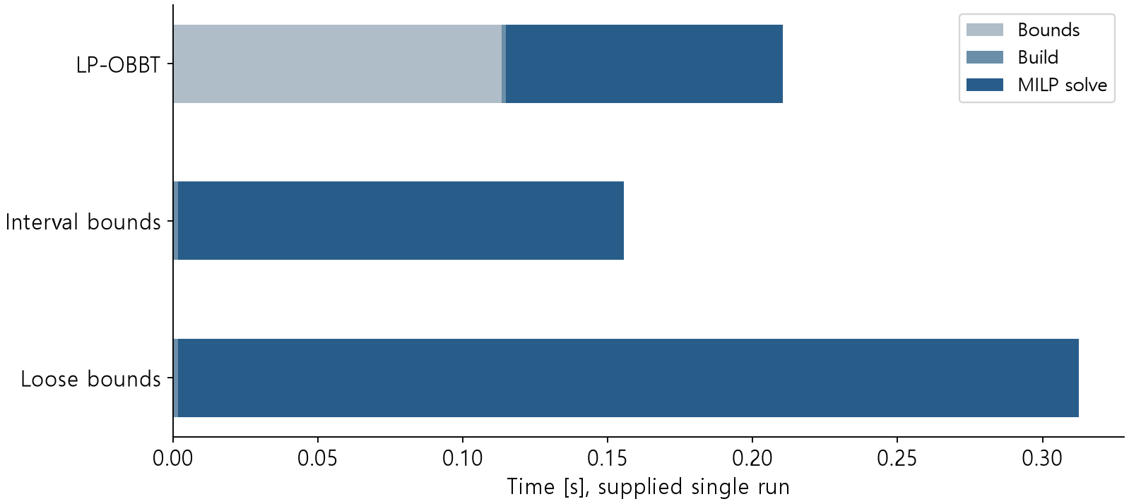
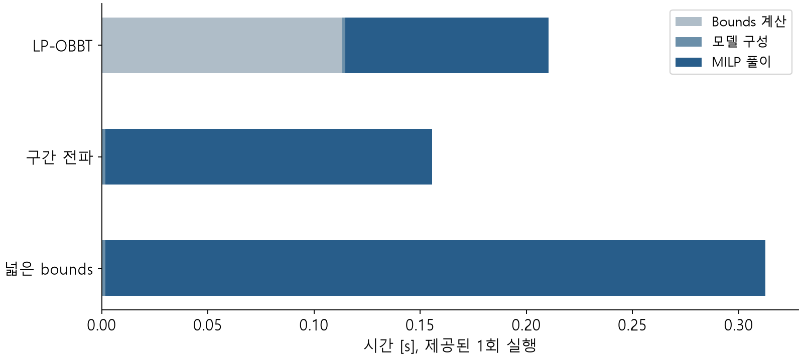
In the supplied run, LP-OBBT reduces MILP solve time, but its total time including bounds exceeds interval propagation. These single-run measurements include interface overhead and do not establish a general speed ranking.
Total time when bounds are reused
In the recorded run, interval-bound MILP time was 0.1539 s and LP-OBBT MILP time was 0.0955 s. OBBT preprocessing required 0.1132 s.
| Solves m | Interval: 0.0001+m×0.1555 | OBBT: 0.1132+m×0.0971 |
|---|---|---|
| 1 | 0.1556 s | 0.2103 s |
| 2 | 0.3111 s | 0.3074 s |
| 5 | 0.7776 s | 0.5987 s |
Each per-solve cost includes 0.0016 s for construction. This arithmetic uses rounded recorded times and assumes identical solve times on every repetition; it is not a repeated timing experiment.
Bounds reusable for fixed weights and input domain spread preprocessing cost across solves. A new model or expanded domain requires renewed bound validation, so this calculation cannot automatically be carried over.
Selected conditions and solver conclusions
| Item | Supplied run |
|---|---|
| Temperature [K] | 342.059300 |
| Residence time [min] | 2.524440 |
| Objective [min-equivalent] | 3.165626 |
| Predicted B [mol/L] | 0.380000 |
| Termination / relative gap | optimal / 0 |
HiGHS establishes optimality for this surrogate MILP within the configured numerical tolerances. The B lower bound is active; the C upper bound has slack.
The objective is 2.524440 + 0.02 × (342.059300−310) = 3.165626. The temperature contribution 0.641186 adds to residence time. Recomputing it checks units and offset handling in the reported solver value.
Checking forward agreement and residuals
Remove product specifications, fix the input, and solve only the network representation. Evaluate the four domain corners and 12 independent interior points with both the hand-built and OMLT models.
Across 32 checks, the maximum absolute output difference is 7.77e-16 mol/L. Recompute the forward pass at the selected optimum too.
Check constraint and integrality residuals. Finite samples help detect implementation errors; equivalence over the entire domain follows from the formulation conditions developed in Week 5.
Define inequality violations to be zero when satisfied: max(0,0.38−B) for B≥0.38 and max(0,C−0.25) for C≤0.25. For binary value z=0.999999, the integrality residual is its distance 0.000001 to the nearest integer 1; compare it with the solver tolerance.
Termination and incumbent availability
| Termination | Interpretation |
|---|---|
| optimal | Completed within gap and numerical tolerances |
| Time limit, incumbent found | Report the feasible solution and remaining gap |
| Time limit, no incumbent | No usable solution has been obtained |
| infeasible | The formulated feasible set is empty |
| unbounded / error | Inspect bounds, objective, logs, and model |
A time limit alone does not establish infeasibility. The lab returns maxTimeLimit with no incumbent at a zero-second limit, and infeasible when B ≥ 2.
Checking solution availability and loading results
opt = Highs()
opt.config.load_solution = False
opt.config.time_limit = 30.0
result = opt.solve(model)
inc = result.best_feasible_objective
print(result.termination_condition)
if inc is not None and np.isfinite(inc):
    result.solution_loader.load_vars()
    print(inc, result.best_objective_bound)
Reading variables after termination without a solution can mistake initial or stale values for results. The complete lab function also returns gaps and constraint residuals.
load_solution=False prevents automatic loading immediately after the solve. Call load_vars only after confirming a finite feasible objective. Then compute specification and integrality residuals from those loaded values.
Solver gaps and process prediction error
| At the same selected input | B concentration [mol/L] |
|---|---|
| Network and MILP | 0.380000 |
| Reference CSTR | 0.371157 |
| Required minimum | 0.380000 |
The reference CSTR misses the B specification. Forward agreement and a zero solver gap still require a separate process-model feasibility check.
Week 8 uses errors at selected points to reconsider decisions and identify additional data.
Running the lab and reporting comparisons
Extract the lab bundle and run these commands in its directory.
python -m pip install -r requirements.txt
python week06_lab.py --output-dir my-results
- Verify the toy LP values 0 and 0.4 and MILP value 0.7 by hand.
- Comparison for the same frozen model: bounds, binary counts, LP lower bounds, and total times
- Report: termination, gap, forward differences, and reference CSTR B-specification violation
Sources and assigned reading
Ceccon et al., OMLT: Optimization & Machine Learning Toolkit, JMLR 23(349), 2022 · Official quick-start