Week 2: Learning Multicomponent Steady-State Responses with MLPs

More conversion does not tell the whole composition

The desired intermediate is B in A → B → C. At short residence time little B forms; at long residence time more B reacts onward to C.

An engineer needs all three outlet concentrations at each condition. One conversion number does not describe the product composition.

Can one model predict A, B, and C consistently?

A process engineer examines the three reactor products A, B, and C.

Three outputs, different errors

All three concentrations have the same units, but their variation differs. An unscaled loss can emphasize one component.

This week learns how an MLP computes these outputs, how one gradient update changes its parameters, and how to evaluate each component.

Learn and check the steady-state MLP

Derive steady-state labels for A, B, and C.
Scale the data and follow a forward pass, backpropagation, and one parameter update.
Train the MLP and compare component RMSE and concentration-sum residuals.

1. A → B → C in a CSTR

Consider a perfectly mixed, constant-volume, constant-density, isothermal CSTR with consecutive first-order reactions A → B → C. The feed contains A; its B and C concentrations are zero. Temperature is an operating input. With concentrations in mol/L, temperature in K, and time in min, the balances are:

\begin{array}{l} \frac{d C_{A}}{d t} = \frac{C_{Af} - C_{A}}{τ} - k_{1} C_{A} \\ \frac{d C_{B}}{d t} = - \frac{C_{B}}{τ} + k_{1} C_{A} - k_{2} C_{B} \\ \frac{d C_{C}}{d t} = - \frac{C_{C}}{τ} + k_{2} C_{B} \end{array}

Rate constants and operating domain

Both rate constants have units of 1/min. Use the following temperature dependence:

\begin{array}{l} k_{1} (T) = 0.2 \exp [6000 (\frac{1}{330} - \frac{1}{T})] \\ k_{2} (T) = 0.1 \exp [5000 (\frac{1}{330} - \frac{1}{T})] \end{array}

Quantity	Value or range
Reference temperature	330 K
Reference k₁; k₂	0.2; 0.1 per minute
Temperature-sensitivity parameters	6000 K; 5000 K
Temperature T	300–360 K
Residence time τ	1–10 min
Feed A concentration	0.8–1.5 mol/L

The three balances describe A consumption, B formation and consumption, and C formation. Adding them cancels the reaction terms.

2. Derive the three-output steady-state map

Set the time derivatives to zero and multiply each balance by τ. Collect the concentration terms:

\begin{array}{l} (1 + k_{1} τ) C_{A} = C_{Af} \\ (1 + k_{2} τ) C_{B} = k_{1} τ C_{A} \\ C_{C} = k_{2} τ C_{B} \end{array}

Solve for A, B, and C

Solve in the order A, B, C:

\begin{array}{l} C_{A} = \frac{C_{Af}}{1 + k_{1} τ} \\ C_{B} = \frac{k_{1} τ C_{Af}}{(1 + k_{1} τ) (1 + k_{2} τ)} \\ C_{C} = k_{2} τ C_{B} \end{array}

At 330 K, τ = 5 min, and feed = 1.2 mol/L, the concentrations are [0.6, 0.4, 0.2] mol/L. Their sum equals the feed concentration. These three outputs are the labels for the steady-state MLP.

Why the B response is nonmonotone

At a fixed temperature, the B yield and its maximizing residence time follow from the expression for C_B:

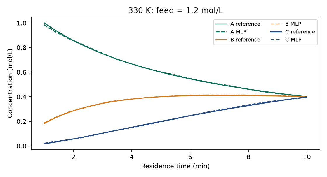
Y_{B} = \frac{C_{B}}{C_{Af}} = \frac{k_{1} τ}{(1 + k_{1} τ) (1 + k_{2} τ)}, τ^{*} = \frac{1}{\sqrt{k_{1} k_{2}}}

Compare the three concentration profiles

At 330 K, τ* is about 7.07 min. Short residence times limit B formation; long residence times allow more B to react to C.

A, B, and C concentration responses to residence time at 330 kelvin, comparing the reference process and MLP. — Three-component response at 330 K. The B concentration has an interior maximum.

3. Prepare the supervised dataset

Each row contains inputs [T, τ, C_Af] and outputs [C_A, C_B, C_C]. Input and output arrays both have shape (N, 3). Generate 400 train, 120 validation, and 160 test operating points within the table’s bounds, then calculate their labels with the steady-state map.

The three concentrations have the same units but different variations. In the training data, their standard deviations are approximately [0.283, 0.110, 0.217] mol/L.

4. Forward calculation and scaling

Use a 3 → 32 → 32 → 3 MLP, with ReLU hidden layers and a linear output layer:

Each hidden layer first computes a weighted sum and bias. ReLU(a) = max(0, a) retains positive values and sets negative values to zero. The weights and biases are the parameters fitted to the concentration data.

\begin{array}{l} h_{1} = ReLU (W_{1} x̃ + b_{1}) \\ h_{2} = ReLU (W_{2} h_{1} + b_{2}) \\ \hat{z} = W_{3} h_{2} + b_{3} \end{array}

Layer	Weight shape	Bias shape	Parameters
Input → hidden 1	32 × 3	32	128
Hidden 1 → hidden 2	32 × 32	32	1056
Hidden 2 → output	3 × 32	3	99
Total			1283

Scaling and the training loss

Scale the inputs with the declared lower and upper bounds. Standardize each output with its training mean μ and standard deviation s, and restore physical units after prediction:

\begin{array}{l} {x̃}_{j} = 2 \frac{x_{j} - l_{j}}{u_{j} - l_{j}} - 1 \\ z_{j} = \frac{y_{j} - μ_{j}}{s_{j}}, {\hat{y}}_{j} = μ_{j} + s_{j} {\hat{z}}_{j} \end{array}

The loss averages squared errors across samples and standardized output components:

L = \frac{1}{3 N} \sum_{n = 1}^{N} \sum_{j = 1}^{3} {({\hat{z}}_{n, j} - z_{n, j})}^{2}

Thus a concentration error is measured relative to that component’s training variation. For example, the smaller B standard deviation gives its raw squared error a larger weight in this loss.

5. Backpropagation: one calculation

Take a 3 → 2 → 3 network with zero biases and the following values. For this calculation, use L = ½‖ŷ − y‖² and learning rate 0.1.

\begin{array}{l} x = [\begin{matrix} 1 \\ 0 \\ -1 \end{matrix}], y = [\begin{matrix} 0 \\ 1 \\ 0 \end{matrix}] \\ W_{1} = [\begin{matrix} 1 & 0 & 0 \\ 0 & 0 & 1 \end{matrix}], W_{2} = [\begin{matrix} 1 & 0 \\ 0 & 1 \\ 1 & 1 \end{matrix}] \end{array}

The hidden pre-activation a, hidden activation h, prediction, and error are:

a = [\begin{matrix} 1 \\ -1 \end{matrix}], h = [\begin{matrix} 1 \\ 0 \end{matrix}], \hat{y} = [\begin{matrix} 1 \\ 0 \\ 1 \end{matrix}], e = [\begin{matrix} 1 \\ -1 \\ 1 \end{matrix}]

Gradients and the parameter update

The output error propagates through the output weights and the ReLU derivative:

\begin{array}{l} δ_{2} = e, \nabla_{W_{2}} L = e h^{T} = [\begin{matrix} 1 & 0 \\ -1 & 0 \\ 1 & 0 \end{matrix}] \\ δ_{1} = ({W_{2}}^{T} e) ⊙ [\begin{matrix} 1 \\ 0 \end{matrix}] = [\begin{matrix} 2 \\ 0 \end{matrix}] \\ \nabla_{W_{1}} L = δ_{1} x^{T} = [\begin{matrix} 2 & 0 & -2 \\ 0 & 0 & 0 \end{matrix}] \end{array}

The bias gradients are δ₁ and δ₂. Update every weight and bias with parameter ← parameter − 0.1 × gradient. The next forward calculation gives [0.26, 0.14, 0.26], and the loss decreases from 1.5 to 0.4374. The notebook checks these gradients using autograd.

6. Train and evaluate the steady-state model

Use Adam with learning rate 0.001, batches of 64, and up to 1400 epochs. After each epoch, evaluate validation loss and retain the weights at its minimum. One batch follows these operations:

prediction = model(inputs)
loss = loss_function(prediction, targets)
optimizer.zero_grad()
loss.backward()
optimizer.step()

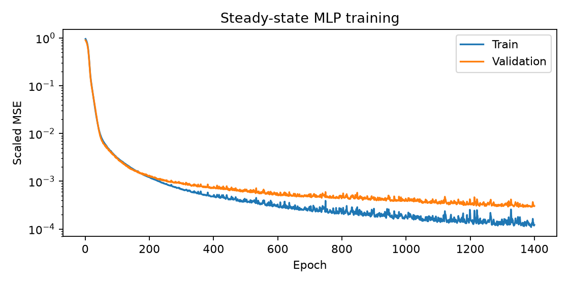
Training and validation scaled mean squared errors for the steady-state MLP. — Training and validation loss. Prediction metrics below are computed after restoring mol/L units.

Evaluate each output component

Test RMSE, mol/L	A	B	C
Output scaling	0.005275	0.002940	0.004423
Unscaled outputs	0.006634	0.003917	0.004162

In this comparison, output scaling reduces A and B RMSE; C RMSE is slightly higher. Evaluate each component rather than combining all three into one error number.

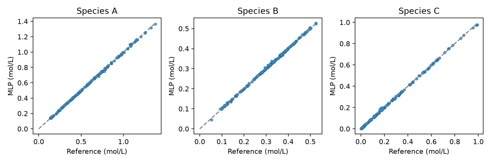
Reference-versus-predicted parity plots for the three concentrations on the test set. — Separate parity plots reveal each component's errors.

Check the concentration sum

Also calculate the concentration-sum residual:

r = \hat{C_{A}} + \hat{C_{B}} + \hat{C_{C}} - C_{Af}

Its test RMSE is 0.003781 mol/L. Component prediction errors and the residual describe different aspects of the model.

The three linear outputs are free predictions. Balance-consistent training labels do not force their sum to match the feed concentration.

For feed 1.2 mol/L, predictions [0.62, 0.41, 0.20] mol/L sum to 1.23 mol/L, giving r = 0.03 mol/L. A model predicting mole fractions can likewise return a sum different from one.

A small prediction error does not enforce a required equality.

Week 4 preview: put the constraint into the model

We can correct a prediction after training, or include a constraint-respecting transformation in the training calculation.

Approach	Where the correction enters
Post-training mapping/projection	Train the raw predictor, then correct its outputs.
KKT-hPINN	Apply a fixed affine projection using the input and raw prediction before the loss, and at inference.

x \to f_{θ} \to \hat{y} \to Π_{x} \to \tilde{y} \to loss

KKT-hPINN computes loss on the projected output and backpropagates through the projection. Its coefficients are fixed; the MLP weights learn with that transformation in place.

Week 4 derives the projection and KKT conditions, checks rank assumptions, and follows the gradient. The guarantee concerns the specified linear equalities, up to numerical arithmetic; nonnegativity needs an additional constraint.

Source: Chen et al. (2024), DOI: 10.1016/j.compchemeng.2024.108764.

7. Run the required steady-state lab

Download the steady-state notebook.

python -m pip install -r requirements.txt
python week02_lab.py --mode steady --output-dir week02-results

Evaluate the trained predictor by component RMSE and concentration-sum residual.

8. Core exercises and submission

Derive C_A, C_B, and C_C and verify their sum. Explain the nonmonotone B curve.
Count the 1283 steady-state MLP parameters and verify the hand-calculated gradient update.
Compare scaled and unscaled outputs by each component’s RMSE.
Inspect concentration-sum residual and minimum predicted concentration on held-out inputs.

Submit the steady-state model, split/scaling details, checked gradient update, and component/consistency evaluation.

Original explanations: PyTorch model construction, autograd, and training.

Reading companion

The Week 2 companion and English PDF explain the three-output map, parameter count, scaling, gradient update, training loop, and independent diagnostics.

KKT-hPINN reference: Chen, H., Constante Flores, G. E., & Li, C. (2024). Physics-informed neural networks with hard linear equality constraints. Computers & Chemical Engineering, 189, 108764.

2주차: MLP로 다성분 정상상태 응답 학습하기

A가 줄어들면 B는 얼마나 만들어질까?

A → B → C에서 원하는 중간 생성물은 B다. 체류시간이 짧으면 B가 충분히 만들어지지 않고, 길면 더 많은 B가 C로 반응한다.

엔지니어는 각 조건에서 세 출구 농도를 알아야 한다. 전환율 하나로는 제품 조성을 설명할 수 없다.

한 모델이 A·B·C를 일관되게 예측할 수 있을까?

출력은 세 개, 오차의 크기도 다르다

세 농도의 단위는 같아도 변화 폭은 다르다. Scaling 없는 loss는 한 성분을 더 강조할 수 있다.

이번 주는 MLP가 출력을 계산하는 방법, 한 번의 gradient 갱신으로 파라미터가 바뀌는 과정, 성분별 평가를 배운다.

정상상태 MLP를 학습하고 확인하기

A·B·C의 정상상태 label을 유도한다.
데이터를 scaling하고 forward·backpropagation·파라미터 갱신 한 번을 따라간다.
MLP를 학습하고 성분별 RMSE와 농도 합 residual을 비교한다.

1. CSTR의 연속반응 A → B → C

완전혼합·일정 부피·일정 밀도·등온 CSTR에서 1차 연속반응 A → B → C를 다룬다. 유입물은 A를 포함하며 B·C의 유입 농도는 0이다. 온도는 운전 입력이다. 농도 단위는 mol/L, 온도는 K, 시간은 min이며 물질수지는 다음과 같다.

\begin{array}{l} \frac{d C_{A}}{d t} = \frac{C_{Af} - C_{A}}{τ} - k_{1} C_{A} \\ \frac{d C_{B}}{d t} = - \frac{C_{B}}{τ} + k_{1} C_{A} - k_{2} C_{B} \\ \frac{d C_{C}}{d t} = - \frac{C_{C}}{τ} + k_{2} C_{B} \end{array}

속도상수와 운전 영역

두 속도상수의 단위는 1/min이다. 온도 의존성은 다음 식을 사용한다.

\begin{array}{l} k_{1} (T) = 0.2 \exp [6000 (\frac{1}{330} - \frac{1}{T})] \\ k_{2} (T) = 0.1 \exp [5000 (\frac{1}{330} - \frac{1}{T})] \end{array}

항목	값·범위
기준 온도	330 K
기준 k₁; k₂	0.2; 0.1 /min
온도 민감도 파라미터	6000 K; 5000 K
온도 T	300–360 K
체류시간 τ	1–10 min
유입 A 농도	0.8–1.5 mol/L

세 수지는 A의 소모, B의 생성·소모, C의 생성을 나타낸다. 세 식을 더하면 반응 항이 상쇄된다.

2. 세 출력을 갖는 정상상태 mapping 유도

시간 미분을 0으로 놓고 각 식에 τ를 곱한다. 농도 항을 모으면 다음 관계를 얻는다.

\begin{array}{l} (1 + k_{1} τ) C_{A} = C_{Af} \\ (1 + k_{2} τ) C_{B} = k_{1} τ C_{A} \\ C_{C} = k_{2} τ C_{B} \end{array}

A·B·C 농도 계산

A, B, C 순서로 풀면 다음과 같다.

\begin{array}{l} C_{A} = \frac{C_{Af}}{1 + k_{1} τ} \\ C_{B} = \frac{k_{1} τ C_{Af}}{(1 + k_{1} τ) (1 + k_{2} τ)} \\ C_{C} = k_{2} τ C_{B} \end{array}

330 K, τ = 5 min, 유입 농도 1.2 mol/L에서는 [0.6, 0.4, 0.2] mol/L이다. 세 농도의 합은 유입 농도와 같다. 이 세 출력을 정상상태 MLP의 label로 사용한다.

B 응답이 단조롭지 않은 이유

고정 온도에서 B의 수율과 이를 최대화하는 체류시간은 C_B 식에서 얻는다.

Y_{B} = \frac{C_{B}}{C_{Af}} = \frac{k_{1} τ}{(1 + k_{1} τ) (1 + k_{2} τ)}, τ^{*} = \frac{1}{\sqrt{k_{1} k_{2}}}

세 성분의 농도 profile 비교

330 K에서 τ*는 약 7.07 min이다. 체류시간이 짧으면 B가 충분히 생성되지 않고, 길면 더 많은 B가 C로 반응한다.

330 K에서 체류시간에 따른 A·B·C 농도와 기준 모델·MLP 비교. — 330 K에서의 다성분 응답. B 농도는 중간 체류시간에서 최대가 된다.

3. 학습 데이터 구성

한 행의 입력은 [T, τ, C_Af], 출력은 [C_A, C_B, C_C]다. 입력·출력 배열의 shape은 모두 (N, 3)이다. 표의 운전 영역에서 train 400개, validation 120개, test 160개를 생성하고 정상상태 식으로 label을 계산한다.

세 농도는 단위가 같지만 변화 폭이 다르다. Train 데이터의 표준편차는 약 [0.283, 0.110, 0.217] mol/L이다.

4. Forward 계산과 scaling

3 → 32 → 32 → 3 MLP를 사용한다. Hidden layer에는 ReLU, 출력층에는 linear 연산을 둔다.

각 hidden layer는 입력의 가중합에 bias를 더한다. ReLU(a) = max(0, a)는 양수 값을 그대로 두고 음수 값을 0으로 만든다. 농도 데이터에 맞춰 학습하는 parameter는 weight와 bias다.

\begin{array}{l} h_{1} = ReLU (W_{1} x̃ + b_{1}) \\ h_{2} = ReLU (W_{2} h_{1} + b_{2}) \\ \hat{z} = W_{3} h_{2} + b_{3} \end{array}

층	Weight shape	Bias shape	Parameter 수
입력 → hidden 1	32 × 3	32	128
Hidden 1 → hidden 2	32 × 32	32	1056
Hidden 2 → 출력	3 × 32	3	99
합계			1283

Scaling과 학습 loss

입력은 명시한 하한·상한으로 scaling한다. 각 출력은 train 평균 μ와 표준편차 s로 표준화하고, 예측 뒤 원래 단위로 되돌린다.

\begin{array}{l} {x̃}_{j} = 2 \frac{x_{j} - l_{j}}{u_{j} - l_{j}} - 1 \\ z_{j} = \frac{y_{j} - μ_{j}}{s_{j}}, {\hat{y}}_{j} = μ_{j} + s_{j} {\hat{z}}_{j} \end{array}

Loss는 표본과 표준화된 출력 성분에 걸쳐 제곱 오차를 평균한다.

L = \frac{1}{3 N} \sum_{n = 1}^{N} \sum_{j = 1}^{3} {({\hat{z}}_{n, j} - z_{n, j})}^{2}

농도 오차를 해당 성분의 train 변화 폭에 상대적으로 평가하는 셈이다. 표준편차가 작은 B의 원래 단위 제곱 오차에는 더 큰 가중치가 붙는다.

5. Backpropagation 한 번 계산하기

Bias가 모두 0인 3 → 2 → 3 신경망에서 다음 값을 사용한다. 이번 계산의 loss는 L = ½‖ŷ − y‖², learning rate는 0.1이다.

\begin{array}{l} x = [\begin{matrix} 1 \\ 0 \\ -1 \end{matrix}], y = [\begin{matrix} 0 \\ 1 \\ 0 \end{matrix}] \\ W_{1} = [\begin{matrix} 1 & 0 & 0 \\ 0 & 0 & 1 \end{matrix}], W_{2} = [\begin{matrix} 1 & 0 \\ 0 & 1 \\ 1 & 1 \end{matrix}] \end{array}

Hidden pre-activation a, activation h, 예측값, 오차는 다음과 같다.

a = [\begin{matrix} 1 \\ -1 \end{matrix}], h = [\begin{matrix} 1 \\ 0 \end{matrix}], \hat{y} = [\begin{matrix} 1 \\ 0 \\ 1 \end{matrix}], e = [\begin{matrix} 1 \\ -1 \\ 1 \end{matrix}]

Gradient와 파라미터 갱신

출력 오차를 출력층 가중치와 ReLU 미분을 거쳐 전달한다.

\begin{array}{l} δ_{2} = e, \nabla_{W_{2}} L = e h^{T} = [\begin{matrix} 1 & 0 \\ -1 & 0 \\ 1 & 0 \end{matrix}] \\ δ_{1} = ({W_{2}}^{T} e) ⊙ [\begin{matrix} 1 \\ 0 \end{matrix}] = [\begin{matrix} 2 \\ 0 \end{matrix}] \\ \nabla_{W_{1}} L = δ_{1} x^{T} = [\begin{matrix} 2 & 0 & -2 \\ 0 & 0 & 0 \end{matrix}] \end{array}

Bias gradient는 각각 δ₁, δ₂다. 모든 weight·bias를 parameter ← parameter − 0.1 × gradient로 갱신한다. 다음 forward의 출력은 [0.26, 0.14, 0.26], loss는 1.5에서 0.4374로 감소한다. Notebook에서 autograd로 이 gradient를 확인한다.

6. 정상상태 모델 학습과 평가

Adam, learning rate 0.001, batch 64, 최대 1400 epoch를 사용한다. 매 epoch 뒤 validation loss를 계산하고 최소값의 가중치를 저장한다. 한 batch의 학습은 다음 연산으로 구성된다.

prediction = model(inputs)
loss = loss_function(prediction, targets)
optimizer.zero_grad()
loss.backward()
optimizer.step()

정상상태 MLP의 train·validation 표준화 MSE 곡선. — Train·validation loss. 아래 예측 지표는 mol/L 단위로 되돌린 뒤 계산한다.

출력 성분별 평가

Test RMSE, mol/L	A	B	C
출력 scaling 적용	0.005275	0.002940	0.004423
출력 scaling 미적용	0.006634	0.003917	0.004162

이 비교에서는 출력 scaling으로 A·B RMSE가 감소하고, C RMSE는 조금 증가했다. 세 오차를 하나로 합치기보다 성분별로 확인한다.

Test 데이터의 A·B·C 농도에 대한 기준값·예측값 parity plot. — 성분별 parity plot에서 각 출력의 오차를 확인한다.

농도 합 확인

농도 합 residual도 계산한다.

r = \hat{C_{A}} + \hat{C_{B}} + \hat{C_{C}} - C_{Af}

Test residual RMSE는 0.003781 mol/L이다. 성분별 예측 오차와 농도 합 residual은 모델의 서로 다른 성질을 보여준다.

세 linear output은 자유롭게 예측된다. 수지를 만족하는 label로 학습해도 예측 농도 합이 유입 농도와 같도록 강제되지는 않는다.

유입 1.2 mol/L에서 예측이 [0.62, 0.41, 0.20] mol/L이면 합은 1.23 mol/L, r = 0.03 mol/L이다. 몰분율을 예측하는 모델에서도 합이 1과 다른 값이 나올 수 있다.

예측 오차가 작다는 것과 반드시 지켜야 할 등식을 만족한다는 것은 다르다.

4주차 예고: 제약을 모델 안에 넣으면?

학습 후 예측을 보정할 수도 있고, 제약을 지키는 변환을 학습 계산 안에 넣을 수도 있다.

접근	보정이 들어가는 위치
학습 후 외부 mapping/projection	Raw predictor를 학습한 뒤 출력을 보정한다.
KKT-hPINN	입력과 raw 예측을 받는 고정 affine projection을 loss 전에 적용하며, 예측할 때도 적용한다.

x \to f_{θ} \to \hat{y} \to Π_{x} \to \tilde{y} \to loss

KKT-hPINN은 projection을 거친 출력으로 loss를 계산하고, projection을 통해 역전파한다. Layer의 계수는 고정되어 있고, MLP의 weight는 이 변환을 반영하여 학습한다.

4주차에서 projection·KKT 조건을 유도하고 rank 가정과 gradient를 확인한다. 보장 범위는 명시한 선형 등식의 만족(수치 연산 오차 범위)이며, 비음수성은 별도 제약이 필요하다.

출처: Chen et al. (2024), DOI: 10.1016/j.compchemeng.2024.108764.

7. 필수 정상상태 실습 실행

정상상태 Notebook을 받는다.

python -m pip install -r requirements.txt
python week02_lab.py --mode steady --output-dir week02-results

학습한 predictor의 성분별 RMSE와 농도 합 residual을 평가한다.

8. 필수 연습문제와 제출물

C_A·C_B·C_C를 유도하고 합을 확인한다. B 곡선이 단조롭지 않은 이유를 설명한다.
정상상태 MLP의 1283개 파라미터와 손 계산한 gradient 갱신을 확인한다.
출력 scaling 적용 전후의 성분별 RMSE를 비교한다.
독립 입력에서 농도 합 residual과 최소 예측 농도를 살펴본다.

정상상태 모델, 분할·scaling 정보, 확인한 gradient 갱신, 성분별 오차·일관성 평가를 제출한다.

원문 해설: PyTorch 모델 구성, autograd, 학습.

읽기자료

2주차 읽기자료와 국문 PDF에서 세 출력 mapping, 파라미터 수, scaling, gradient 갱신, 학습 loop와 독립 진단을 읽는다.

KKT-hPINN 참고문헌: Chen, H., Constante Flores, G. E., & Li, C. (2024). Physics-informed neural networks with hard linear equality constraints. Computers & Chemical Engineering, 189, 108764.