Week 1: From Process Prediction to Decisions

Learning objectives

After this lesson, you should be able to write the inputs, outputs, fixed context, units, and operating domain of a surrogate; distinguish training from operational optimization; construct a steady-state and a dynamic CSTR example; and check whether a surrogate-selected operating point satisfies the reference model’s constraints.

1. Begin with the decision

Suppose a reactor operator wants high conversion at a low operating cost. Predicting conversion at a proposed temperature is one task. Choosing temperature and residence time while meeting a conversion requirement is another task. The second task repeatedly queries the model in regions favored by the optimizer, which may differ from a typical held-out test sample.

Write four items before selecting a network: what can be changed, what is fixed for this decision, what must be predicted, and what counts as a satisfactory operating point. A small prediction error averaged across the domain does not tell us whether a constraint is satisfied at the selected point.

Role	Meaning	Example in this lesson
Decision variables	Quantities selected by the optimization	Reactor temperature T and residence time τ
Fixed context	Known quantities held fixed for one solve	Feed concentration set to 1.2 mol/L for the decision comparison
Model outputs	Quantities predicted for a proposed input	Outlet concentration and conversion
State	A quantity that evolves in a dynamic model	Reactor concentration
Domain	Conditions over which the model is evaluated	Stated bounds on temperature, residence time, and feed concentration

Training adjusts model parameters using data. Operational optimization holds the trained parameters fixed and changes the decision variables. These are different optimization problems.

2. A reference process we can check

Use an ideal, perfectly mixed, constant-volume, isothermal CSTR with a first-order reaction A → B, constant density, and no B in the feed. Reactor temperature T is an operating input.

\frac{d C_{A}}{d t} = \frac{C_{A f} - C_{A}}{τ} - k (T) C_{A}

Here concentrations are in mol/L, time and residence time in minutes, T in kelvin, and k in inverse minutes. The flow-to-volume ratio is the reciprocal of residence time. The inlet–outlet term and the reaction term therefore both have units of mol/(L·min).

The rate constant depends on temperature as follows:

k (T) = k_{ref} \exp [β (\frac{1}{T_{ref}} - \frac{1}{T})]

Parameter or input	Value or range	Interpretation
Reference rate constant	0.2 per minute	Rate at the reference temperature
Reference temperature	330 K	Rate-law reference
β = E/R	6000 K	Synthetic temperature-sensitivity parameter
Temperature	300–360 K	Sampling and decision domain
Residence time	1–10 min	Sampling and decision domain
Feed A concentration	0.8–1.5 mol/L	Sampling domain; fixed to 1.2 for optimization

3. Derive the steady-state map

Set the time derivative to zero, multiply by residence time, and collect the terms containing outlet concentration. The resulting mapping and conversion are:

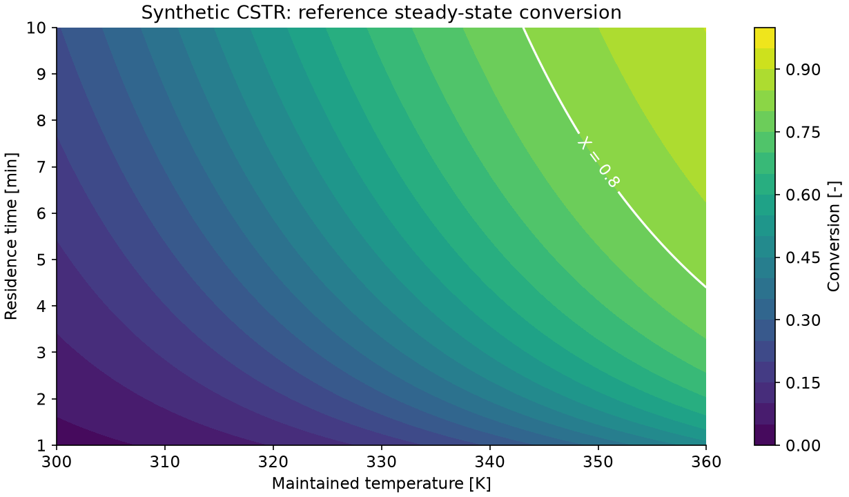
C_{A} = \frac{C_{A f}}{1 + k (T) τ}, X = 1 - \frac{C_{A}}{C_{A f}} = \frac{k (T) τ}{1 + k (T) τ}

This gives a three-input, two-output map: temperature, residence time, and feed concentration map to outlet concentration and conversion. In this first-order model, conversion is independent of feed concentration.

A worked check: at 330 K and 5 min, the product kτ is 1, so conversion is 0.5 and outlet A concentration is half the inlet concentration. For the 1.2 mol/L feed, the outlet is 0.6 mol/L.

Reference CSTR conversion across temperature and residence time, with the 0.8 conversion contour. — Reference-model conversion. The contour marks the conversion requirement used in the decision exercise.

4. State the optimization problem

Minimize the following dimensionless operating-cost index:

J (T, τ) = \frac{T - 300 K}{20 K} + \frac{τ}{10 min}

The index penalizes higher temperature and longer residence time. At a fixed feed concentration of 1.2 mol/L, minimize this index over the stated bounds subject to predicted conversion of at least 0.8. Also require predicted concentration to lie between zero and the feed concentration, and predicted conversion not to exceed one.

For the reference map, conversion of at least 0.8 is equivalent to kτ of at least 4. This follows by multiplying the conversion inequality by the positive denominator. It gives a useful independent check on the feasible region.

Surrogate prediction errors can change the feasible set. Run the selected temperature and residence time through the reference model and check whether the conversion requirement is met.

5. Design data for the intended use

The lab generates 400 training, 120 validation, and 160 test points independently inside the stated box, using a fixed random seed. Fit model coefficients using training data, use validation for model choices, and reserve the test set for reporting. The baseline uses fixed domain scaling and quadratic features.

The two-output baseline uses ordinary least-squares regression on ten features: a constant, three scaled inputs, their squares, and their pairwise products.

Split measured data by batch, experiment, campaign, or time. For dynamic data, split by entire trajectories so that overlapping windows remain in the same split.

6. Prediction error and decision error

Report concentration RMSE in mol/L and conversion RMSE as a dimensionless fraction. Also report the consistency residual relating the two outputs: predicted outlet concentration plus feed concentration times predicted conversion minus feed concentration. A multi-output fit can disagree with this identity.

The decision comparison enumerates the same grid for the surrogate and reference maps: temperature steps of 0.5 K and residence-time steps of 0.1 min. It finds the lowest-cost feasible candidate on that grid.

Check	Result
Held-out concentration RMSE	0.032623 mol/L
Held-out conversion RMSE	0.025608
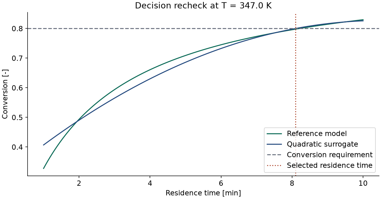
Selected surrogate decision	347.000000 K; 8.100000 min
Predicted conversion at that decision	0.800144
Reference conversion at that decision	0.797893
Reference conversion shortfall below 0.8	0.002107
Reference cost of the surrogate-selected decision	3.160000
Reference-model feasible grid benchmark cost	3.155000

At the selected point, the surrogate predicts conversion above 0.8, while the reference model falls below 0.8. This point violates the conversion constraint. Compare costs among points that pass the reference feasibility check.

Reference and surrogate conversion along residence time at the selected temperature, with the conversion target. — A local check near the selected decision. Error close to the constraint boundary can change the feasible operating choices.

7. Connect vectors to time series

A steady-state output has no time index. A dynamic output depends on the initial state and the history of control inputs and disturbances. In a planning problem, the model must also receive the future control sequence being considered; predicting from historical measurements alone is insufficient to compare arbitrary future control plans.

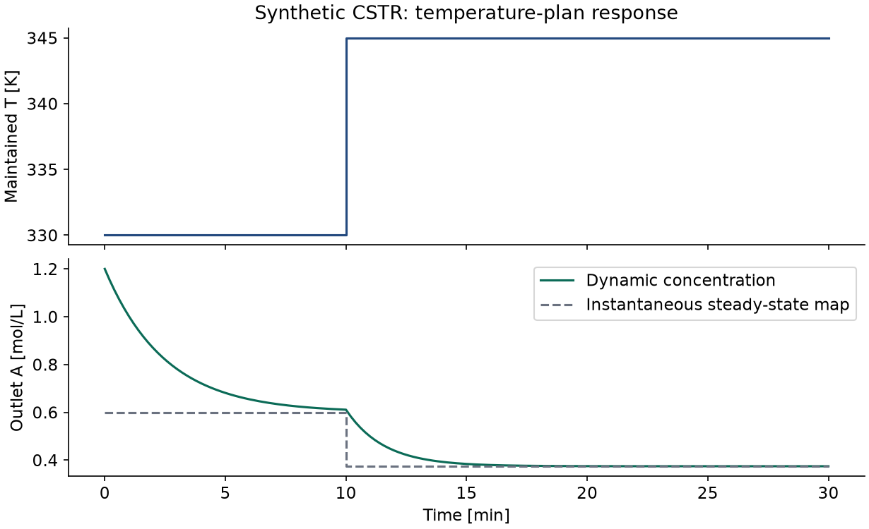
The dynamic lab holds the feed concentration and residence time fixed and changes the maintained temperature from 330 to 345 K at 10 min. Within each constant-input interval, the concentration balance has an analytic update:

C_{A} (t + Δ t) = C_{A ss} + [C_{A} (t) - C_{A ss}] \exp [- (\frac{1}{τ} + k (T)) Δ t]

For each interval, calculate the steady-state concentration using that interval’s inputs.

The code records input values on intervals and concentration on interval boundaries. At the step time, the concentration is continuous and then approaches the new steady value.

Maintained reactor temperature and concentration response to a temperature step at ten minutes. — Dynamic reference response. An instantaneous steady-state mapping would miss the transient concentration trajectory.

8. Run the lab

Download the notebook or the standalone script, plus requirements.txt.

python -m pip install -r requirements.txt
python week01_lab.py --output-dir week01-results

The script creates the dataset, metrics JSON, dynamic trajectory CSV, and three figures inside the chosen output directory. The published dataset and recorded results are also available for comparison.

9. Exercises and submission

Derive the steady-state concentration and check its units. Explain why increasing either temperature or residence time increases conversion under this model.
Derive the condition kτ ≥ 4 for the conversion target. Check the reference feasible region without fitting a model.
Re-run the lab with a different training seed. Compare test RMSE, the selected operating point, and reference feasibility. Does better RMSE always select a better decision?
Tighten the temperature domain to 330–350 K. Explain how the feasible set and the sampled training domain should change together.
Change the temperature step time. Describe which input intervals and output boundary times change. Explain why a steady-state predictor cannot represent the transient.
Write a one-page problem specification stating the decision variables, fixed context, state, outputs, units, domain, objective, constraints, data split, and revalidation rule.

Reference checks: at 330 K and 5 min, conversion is 0.5; the conversion target requires kτ ≥ 4; increasing T increases k for positive β. The other exercises require your computed results and interpretation, including failed constraints when they occur.

Reading and next lesson

Read selected parts of Boyd and Vandenberghe’s Chapters 2–4 on domains, constraints, convex functions, and optimization problems. Read the OMLT introduction for the role of trained models in larger optimization problems.

Week 2 builds a multi-output MLP using the same data definition and reference checks.

학습 목표

이 강의를 마치면 surrogate의 입력, 출력, 고정 context, 단위, 운전 영역을 정의하고, 학습과 운전 최적화를 구분하며, 정상상태·동적 CSTR 예제를 구성하고, surrogate가 선택한 운전점이 기준 모델의 제약을 만족하는지 확인할 수 있어야 한다.

1. 의사결정 문제에서 시작하기

반응기 운전자가 비용을 낮추면서 높은 전환율을 얻고 싶다고 하자. 주어진 온도에서 전환율을 예측하는 일과, 전환율 요구를 만족하도록 온도·체류시간을 선택하는 일은 다르다. 후자는 optimizer가 선호하는 영역에서 모델을 반복해서 평가한다. 그 영역은 일반적인 독립 test 표본의 분포와 다를 수 있다.

신경망을 고르기 전에 무엇을 바꿀 수 있는지, 이번 결정에서 무엇이 고정되는지, 무엇을 예측해야 하는지, 어떤 운전점을 받아들일 것인지부터 작성한다. 영역 전체의 평균 예측 오차가 작다고 해서 선택한 운전점이 제약을 만족하는 것은 아니다.

역할	의미	이번 예제
의사결정 변수	최적화가 선택하는 양	반응기 온도 T와 체류시간 τ
고정 context	한 번의 solve에서 고정하는 알려진 양	의사결정 비교에서는 유입 농도 1.2 mol/L
모델 출력	제안된 입력에서 예측하는 양	출구 농도와 전환율
상태	동적 모델에서 시간에 따라 변하는 양	반응기 내부 농도
영역	모델을 평가할 조건의 범위	온도·체류시간·유입 농도의 명시된 bounds

학습은 데이터를 이용해 모델 파라미터를 조정한다. 운전 최적화는 학습된 파라미터를 고정하고 의사결정 변수를 바꾼다. 서로 다른 최적화 문제다.

2. 직접 확인할 수 있는 기준 공정

1차 반응 A → B가 일어나는 이상적인 완전혼합·일정 부피·등온 CSTR를 사용한다. 밀도는 일정하고 유입물에는 B가 없다. 반응기 온도 T를 조작변수로 둔다.

\frac{d C_{A}}{d t} = \frac{C_{A f} - C_{A}}{τ} - k (T) C_{A}

농도 단위는 mol/L, 시간과 체류시간은 min, T는 K, k는 1/min이다. 유량/부피는 체류시간의 역수이므로 유입–유출 항과 반응 항의 단위는 모두 mol/(L·min)이다.

속도상수의 온도 의존성은 다음과 같다.

k (T) = k_{ref} \exp [β (\frac{1}{T_{ref}} - \frac{1}{T})]

파라미터·입력	값·범위	의미
기준 속도상수	0.2 /min	기준 온도에서의 속도
기준 온도	330 K	속도식의 기준
β = E/R	6000 K	교육용 온도 민감도 파라미터
온도	300–360 K	Sampling·의사결정 영역
체류시간	1–10 min	Sampling·의사결정 영역
유입 A 농도	0.8–1.5 mol/L	Sampling 영역; 최적화에서는 1.2로 고정

3. 정상상태 mapping 유도

시간 미분을 0으로 놓고 체류시간을 곱한 뒤 출구 농도가 들어 있는 항을 모은다. 정상상태 mapping과 전환율은 다음과 같다.

C_{A} = \frac{C_{A f}}{1 + k (T) τ}, X = 1 - \frac{C_{A}}{C_{A f}} = \frac{k (T) τ}{1 + k (T) τ}

온도·체류시간·유입 농도라는 세 입력에서 출구 농도·전환율이라는 두 출력을 얻는다. 이 1차 반응 모델에서 전환율은 유입 농도에 무관하다.

계산 확인: 330 K, 5 min에서는 kτ가 1이므로 전환율은 0.5이고 출구 A 농도는 유입 농도의 절반이다. 유입이 1.2 mol/L이면 출구는 0.6 mol/L이다.

온도와 체류시간에 따른 기준 CSTR 전환율 및 전환율 0.8의 contour. — 기준 모델의 전환율. Contour는 의사결정 실습에서 사용할 전환율 요구를 나타낸다.

4. 최적화 문제 명시하기

다음 무차원 비용 지수를 최소화한다.

J (T, τ) = \frac{T - 300 K}{20 K} + \frac{τ}{10 min}

높은 온도와 긴 체류시간에 비용을 부여한다. 유입 농도를 1.2 mol/L로 고정하고, 명시된 bounds 안에서 예측 전환율이 0.8 이상이 되도록 이 지수를 최소화한다. 예측 농도는 0과 유입 농도 사이, 예측 전환율은 1 이하라는 조건도 둔다.

기준 mapping에서는 전환율 0.8 이상이 kτ ≥ 4와 동치다. 전환율 부등식의 양변에 양수인 분모를 곱하면 확인할 수 있다. 모델을 학습하지 않고도 feasible region을 확인하는 기준이다.

Surrogate의 예측 오차로 feasible set이 달라질 수 있다. 선택한 온도·체류시간을 기준 모델에 넣고 전환율 요구를 만족하는지 확인한다.

5. 사용할 목적에 맞는 데이터 설계

실습은 고정 random seed로 명시된 box 안에서 train 400개, validation 120개, test 160개를 독립 생성한다. Train 데이터로 계수를 학습하고, validation은 모델 선택에, test는 최종 평가에 사용한다. Baseline은 고정 영역 scaling과 quadratic feature를 사용한다.

다출력 baseline은 상수항, 세 scaled 입력, 각 입력의 제곱, 입력 사이의 곱으로 구성된 열 개 feature에 대한 ordinary least squares를 사용한다.

측정 데이터는 batch, 실험, 운전 campaign, 시간 단위로 분할한다. 동적 데이터는 같은 궤적의 겹치는 window가 한 분할에 속하도록 전체 궤적 단위로 나눈다.

6. 예측 오차와 의사결정 오차

농도 RMSE는 mol/L, 전환율 RMSE는 무차원 비율로 보고한다. 두 출력의 일관성 residual도 확인한다. 예측 출구 농도에 유입 농도×예측 전환율을 더하고 유입 농도를 빼면 된다. 다출력 fit이 이 관계를 만족하지 않을 수 있다.

의사결정 비교는 surrogate와 기준 모델에 동일한 grid를 사용한다. 온도 간격은 0.5 K, 체류시간 간격은 0.1 min이다. 이 grid에서 비용이 가장 작은 feasible 후보를 찾는다.

확인 항목	결과
독립 test 농도 RMSE	0.032623 mol/L
독립 test 전환율 RMSE	0.025608
Surrogate가 선택한 운전점	347.000000 K; 8.100000 min
그 지점의 예측 전환율	0.800144
그 지점의 기준 모델 전환율	0.797893
기준 모델에서 0.8 대비 전환율 부족분	0.002107
선택한 운전점의 기준 비용	3.160000
기준 모델 feasible grid benchmark 비용	3.155000

선택한 운전점의 예측 전환율은 0.8 이상이지만, 기준 모델 전환율은 0.8보다 낮다. 이 운전점은 전환율 제약을 위반한다. 비용은 기준 모델에서 feasible인 운전점 사이에서 비교한다.

선택한 온도에서 체류시간에 따른 기준 전환율·surrogate 전환율과 목표 전환율 비교. — 선택한 운전점 근처의 비교. 제약 경계 근처 오차가 선택 가능한 운전 조건을 바꿀 수 있다.

7. 변수 벡터에서 시간 시계열로 연결하기

정상상태 출력에는 시간 index가 없다. 동적 출력은 초기 상태와 조작변수·외란의 이력에 의존한다. 운전 계획 문제에서는 검토하는 미래 조작변수 sequence도 모델이 입력으로 받아야 한다. 과거 관측만으로 예측하는 모델은 임의의 미래 운전 계획을 비교하기에 충분하지 않다.

동적 실습에서는 유입 농도·체류시간을 고정하고 10 min에 유지 온도를 330 K에서 345 K로 바꾼다. 각 입력이 일정한 구간에서 농도 수지는 다음 해석적 update를 갖는다.

C_{A} (t + Δ t) = C_{A ss} + [C_{A} (t) - C_{A ss}] \exp [- (\frac{1}{τ} + k (T)) Δ t]

각 구간의 정상상태 농도는 해당 구간의 입력으로 계산한다.

코드는 입력을 구간마다, 농도를 구간 경계 시점마다 기록한다. 온도가 바뀌는 순간 농도는 연속이며 이후 새로운 정상값에 접근한다.

10분에 온도를 바꾼 뒤 유지 온도와 반응기 농도의 시간 응답. — 기준 동적 응답. 즉시 정상상태 값을 반환하는 mapping은 과도 농도 궤적을 놓친다.

8. 실습 실행

Notebook 또는 독립 스크립트와 requirements.txt를 받는다.

python -m pip install -r requirements.txt
python week01_lab.py --output-dir week01-results

스크립트는 지정한 출력 폴더에 dataset, metrics JSON, 동적 궤적 CSV, 그림 세 개를 생성한다. 비교를 위한 공개 dataset과 기록된 결과도 제공한다.

9. 연습문제와 제출물

정상상태 농도를 유도하고 단위를 확인한다. 이 모델에서 온도 또는 체류시간을 높이면 전환율이 증가하는 이유를 설명한다.
전환율 목표의 조건 kτ ≥ 4를 유도한다. 모델을 학습하지 않고 기준 feasible region을 확인한다.
Training seed를 바꾸어 다시 실행한다. Test RMSE, 선택한 운전점, 기준 feasibility를 비교한다. RMSE가 더 좋은 모델이 항상 더 좋은 결정을 선택하는가?
온도 영역을 330–350 K로 좁힌다. Feasible set과 training sampling 영역을 어떻게 함께 바꿔야 하는지 설명한다.
온도 step 시점을 바꾼다. 입력 구간과 출력 경계 시점 중 무엇이 달라지는지 설명한다. 정상상태 predictor가 과도 응답을 표현할 수 없는 이유를 설명한다.
의사결정 변수, 고정 context, 상태, 출력, 단위, 영역, 목적함수, 제약, 데이터 분할, 재검증 규칙을 포함한 한 쪽짜리 문제 정의서를 작성한다.

기준 확인: 330 K·5 min의 전환율은 0.5이고, 목표 전환율은 kτ ≥ 4를 요구하며, 양수 β에서는 T가 증가하면 k가 증가한다. 나머지 문제는 직접 계산한 결과와 해석을 제출하며, 제약을 위반했다면 그 결과도 포함한다.

읽기자료와 다음 강의

Boyd와 Vandenberghe의 2–4장 중 domain, 제약, convex function, 최적화 문제 관련 내용을 읽는다. OMLT 서론에서는 큰 최적화 문제 안에 학습된 모델을 넣는 역할을 확인한다.

2주차에서는 같은 데이터 정의와 기준 확인 절차를 사용해 다출력 MLP를 만든다.