Week 7: Designing Model Structure for Optimization
Utility cost models and repeated operating decisions
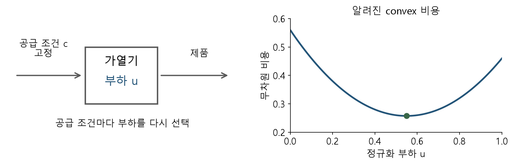
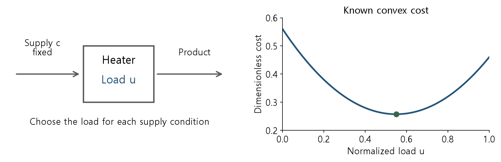
A changing supply condition requires a new heating-load decision. When a neural network predicts the cost curve, its structure also affects the optimization used to select the load.
Goal: load selection with preserved convex cost structure.
Model choice and optimization formulations
Weeks 5 and 6 represented a fitted general ReLU network exactly as an MILP. This week imposes convexity in selected inputs during model design.
We begin with a known convex cost. Reactor concentrations and yields are not assumed convex.
Structural restrictions reduce the function class, so evaluate prediction error together with the resulting decisions.
Learning objectives and deliverables
- Decisions, fixed context, and ICNN sign conditions
- Objective-value equivalence and conditions for a ReLU epigraph LP
- Counterexamples: inequality direction, negative weights, and variable context
- Fitted ICNN decision validation: forward evaluation and reference function
Decision variables and fixed context
Choose a normalized heating load u, while fixing measured supply composition or ambient conditions c. Freeze model parameters θ before optimization.
Convexity here concerns u. It does not establish convexity in c or θ.
c is the observed supply condition; u is the load selected now. A changed supply condition may change the cost curve, so fix the new c and solve again. Distinguish training parameters θ from the operating decision u.
Convex functions and sublevel sets
A convex function lies below the line segment joining two function values.
For convex f, the constraint f(u) ≤ b defines a convex set. The reverse inequality generally does not. This distinction determines valid LP uses.
Boyd and Vandenberghe, Convex Optimization, §§3.1-3.2 and 4.1-4.3
If two inputs each satisfy cost cap b, the cost at their mixture is at most their weighted average and hence at most b. This proves convexity of the sublevel set. The same inequality argument does not establish a lower-cost constraint.
ICNN input connections and sign conditions
Constrain every entry of W and w to be nonnegative. Direct input weights A and a, and biases, may have either sign.
ReLU is convex and nondecreasing. These conditions preserve convexity in the inputs through the layers and output.
Amos, Xu and Kolter, Input Convex Neural Networks, ICML 2017, pp. 146-155
Nonnegative sums preserve the convexity inequality of previous-layer functions. A negative multiplier reverses that inequality. Direct affine input terms have no curvature even with negative slopes, so their weights need no such restriction.
Layerwise convexity derivation
The first layer is a maximum of an affine function and zero, so it is convex. Assume every component of the previous layer is convex.
With W ≥ 0, their weighted sum is convex; adding an affine input connection preserves this property. Applying convex, nondecreasing ReLU preserves it again.
The output condition w ≥ 0 serves the same purpose. Negative slopes in direct input connections remain affine and do not break the argument.
The induction hypothesis is componentwise convexity of the previous layer. Multiplying its inequalities by nonnegative W entries and adding preserves their direction. Applying nondecreasing ReLU then preserves the ordering needed for the composition argument.
Negative weights and input convexity
Negative weights on hidden activations remove the sufficient condition.
Direct input weights need not be nonnegative: ReLU(−u + 0.4) is still convex. Identify which connection each restricted weight belongs to.
Sign constraints during training
After a gradient update, project W to max(W, 0), or parameterize W = softplus(V) using free parameters V. Apply the same rule to output weights w.
Here softplus parameterizes positive weights. Hidden activations remain ReLU during inference.
Inspect the actual fitted weights. Training a general deep ICNN in its parameters is nonlinear and nonconvex.
If an updated constrained weight is −0.03, clipping replaces it by zero; a weight of 0.2 stays unchanged. These restrictions make the function convex in its input, without making the general weight-training problem convex.
ReLU graphs and epigraphs
The two inequalities describe the region above ReLU. They allow h = 10 at s = 0, so they do not represent the graph equality itself.
To use these lower bounds in an LP, it must be possible to reduce the auxiliary activations to the actual outputs, and the objective and remaining constraints must permit that reduction.
At fixed input, values above the true ReLU still satisfy both lower inequalities. Reducing h to its forward value is harmless only when the objective favors reduction and other constraints permit it. These conditions justify using the epigraph instead of the graph equality.
An extended LP for a ReLU ICNN
Constraint scope: a finite ReLU network with frozen weights
Add Gu ≤ r and minimize t. With W, w ≥ 0 and linear remaining expressions, this is an LP without binary variables.
Replacing the activation by softplus can preserve convexity, but not an exact representation by these finitely many linear constraints.
Auxiliary t is an upper value for cost. Every feasible point has t≥f(u), and the actual forward values permit t=f(u). Minimizing t therefore attains the same optimal value as minimizing the original cost.
Forward recovery and objective-value equivalence
At fixed u, a feasible first-layer h dominates the actual ReLU output. Induction using W ≥ 0 gives the same result at every layer, hence t ≥ f(u).
Conversely, the true forward activations with t = f(u) satisfy every constraint. These two inclusions establish the exact epigraph.
The optimum of min t agrees with the objective at the selected u. Auxiliary variables that do not affect the output may remain slack even at an optimum.
Restoring two auxiliary layers to forward values
Consider h₁=ReLU(u−0.4), h₂=ReLU(2h₁−0.1), and f=0.2−u+3h₂. Hidden weight 2 and output weight 3 are positive. Fix u=0.6.
| State | h₁ | h₂ | Output expression |
|---|---|---|---|
| Actual forward | 0.2 | 0.3 | 0.5 |
| Loose epigraph point | 0.4 | 0.7 | 1.7 |
| Restore first layer only | 0.2 | 0.7 | 1.7 |
| Restore second layer | 0.2 | 0.3 | 0.5 |
Lowering h₁ lowers 2h₁−0.1, so the existing h₂ still satisfies its lower bound. Lowering h₂ then decreases the objective because its output coefficient is positive. This is the layer-by-layer restoration argument.
With output coefficient −3, raising h₂ would improve the objective and the argument would fail. An external requirement h₂≥0.7 would also prevent restoration to 0.3. Both weight signs and external constraints matter.
Applicability by output use
| Output use | Assessment |
|---|---|
| min f(u) | Use an epigraph objective |
| f(u) ≤ b | Adding t ≤ b gives the exact input feasible set |
| f(u) ≥ b | Adding only t ≥ b does not enforce a lower bound on the true output |
| y = f(u) | The output graph equality is generally nonconvex |
| max f(u) | The same LP argument does not cover convex maximization |
Also inspect any other constraints that favor larger h or t.
An upper cap gives f(u)≤t≤b and therefore enforces the original cap. A lower bound t≥b can be met by inflating t even when f(u) is small. The same predictor needs different formulations depending on whether its output is minimized, capped, or lower-bounded.
A two-hinge cost model for hand calculation
Dimensionless cost example for direct numerical checks. Successive slopes: −0.6 → 0.4 → 0.9.
Minimum: first slope change at u = 0.4; f(0.4) = 0.16.
Before u=0.4 both ReLUs are zero and the slope is −0.6. Activating the first adds slope 1, giving 0.4; activating the second adds 0.5, giving 0.9. The first knot where cost switches from decreasing to increasing is the minimum.
The hand model LP and a cost cap
A cost cap of 0.25 leaves the feasible input interval [0.25, 0.625]. Bound the affine output expression above to obtain this interval in the LP.
Lab checks: minimum value 0.16 and forward agreement.
Cost and feasibility between two knots
Keep only active ReLUs in each interval to simplify the cost.
| u interval | Active terms | Cost | Condition for f(u)≤0.25 |
|---|---|---|---|
| 0–0.4 | None | 0.4−0.6u | u≥0.25 |
| 0.4–0.7 | u−0.4 | 0.4u | u≤0.625 |
| 0.7–1 | Both | 0.9u−0.35 | u≤2/3, outside this interval |
The feasible interval is [0.25,0.625]. At minimum u=0.4, both ReLUs are zero and f=0.4−0.6×0.4=0.16.
For example, u=0.6 gives h₁=0.2,h₂=0 and f=0.4−0.36+0.2=0.24. This matches 0.4u=0.24 in the middle interval, checking the piecewise expression against the original network.
LP matrix columns and inequalities
Fix variable order [u,h₁,h₂]. Each row of linprog’s A_ub is dotted with the variable vector and bounded above by the matching b_ub entry.
| Code value | Expression | Role |
|---|---|---|
| Objective [−0.6,1,0.5] | −0.6u+h₁+0.5h₂ | Cost without constant 0.4 |
| Row [1,−1,0], rhs 0.4 | u−h₁≤0.4 | h₁≥u−0.4 |
| Row [1,0,−1], rhs 0.7 | u−h₂≤0.7 | h₂≥u−0.7 |
| h bounds (0,None) | h₁,h₂≥0 | Other ReLU lower bounds |
At solution [0.4,0,0], row values [0.4,0.4] satisfy their upper bounds. Add constant 0.4 to solver objective −0.24 to report 0.16. The original forward cost must also be 0.16.
Positive h coefficients make this objective minimize h. Changing their signs requires rechecking the recovery argument.
A counterexample for an output lower bound
On 0 ≤ u ≤ 1, let f(u) = ReLU(u) and minimize u subject to f(u) ≥ 0.8. The true optimum is u = 0.8.
The relaxation permits u = 0, h = 0.8. An inflated auxiliary variable lowers the cost. A small MIP gap or an LP optimal status cannot detect this modeling error.
At u=0,h=0.8, all three linear inequalities hold but f(0)=0. Solving a model with the wrong output lower-bound representation exactly still returns the wrong input. This is why forward validation follows status checking.
Counterexamples for output rewards and graph equalities
Minimizing −h for the same ReLU makes the epigraph LP unbounded when h has no upper bound. The actual f(u) lies in [0, 1], and min −f(u) = −1.
For f(u) = |u|, graph points (−1, 1) and (1, 1) have midpoint (0, 1), which is not on the graph.
Transferring cost-epigraph equivalence directly to concentration equalities or output rewards changes the problem.
PICNNs and fixed context
A PICNN imposes convexity on only part of its input. The path processing supply context c may be nonlinear, while the decision path in u must satisfy the required sign conditions after c is fixed.
The next page uses a sufficient form in which context determines layer coefficients. The paper’s gated construction can also be interpreted this way at fixed context.
Amos, Xu and Kolter, Input Convex Neural Networks, ICML 2017, pp. 146-155
Conditional coefficients and LP construction
Evaluate the context path once at observed c, then freeze its coefficients. With linear remaining decision expressions and constraints, construct the ReLU epigraph LP.
Optimizing c as well can introduce nonlinear products W(c)h or A(c)u. Fixed-context results do not imply joint convexity or an LP.
At observed c, W(c), A(c), and b(c) are numbers. Freezing them makes each expression affine in u and h. Leaving c variable turns a numerical coefficient times a variable into a function of a variable times another variable, which is no longer the same LP.
Conditional versus joint convexity
At fixed c, the optimum is u = c. The lab solves separate LPs for c = 0.2, 0.5, and 0.8.
Along u = c, f = −0.1c². The endpoint average is −0.05 but the midpoint value is −0.025, violating joint convexity.
For fixed c=0.2, represent with t≥u−0.2 and t≥0.2−u, and minimize t−0.004. The minimum is −0.004 at u=0.2,t=0. If c becomes a variable, −0.1c² is no longer a constant, so this LP no longer applies unchanged.
Fitting a known convex reference function
Fit coefficients at 41 evenly spaced inputs and evaluate at 200 separate midpoint inputs. With fixed knots, this lab uses bounded linear least squares.
This shallow ICNN with fixed knots is a special case with convex training. The conclusion does not extend to general deep-ICNN training.
Fixed knots κ allow every ReLU feature to be computed before fitting. Only b,a,w remain unknown, giving bounded linear least squares. w≥0 prevents downward slope jumps at knots and preserves convexity of the fitted curve.
At u=0.25, the feature row is [1,0.25,0.15,0.05,0,0,0,0,0,0,0]. Only knots 0.1 and 0.2 have been crossed. Fit least squares with b and a unrestricted and lower bounds of zero on the remaining nine weights.
Fitted curve and selected load
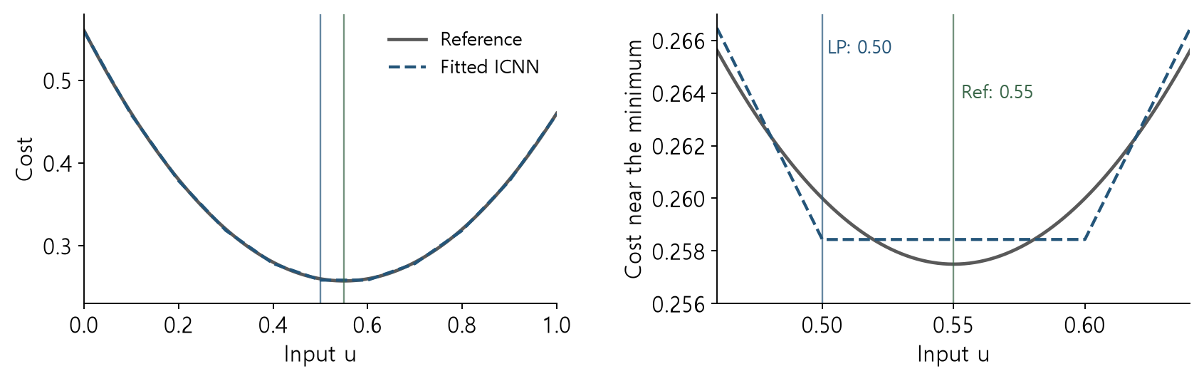
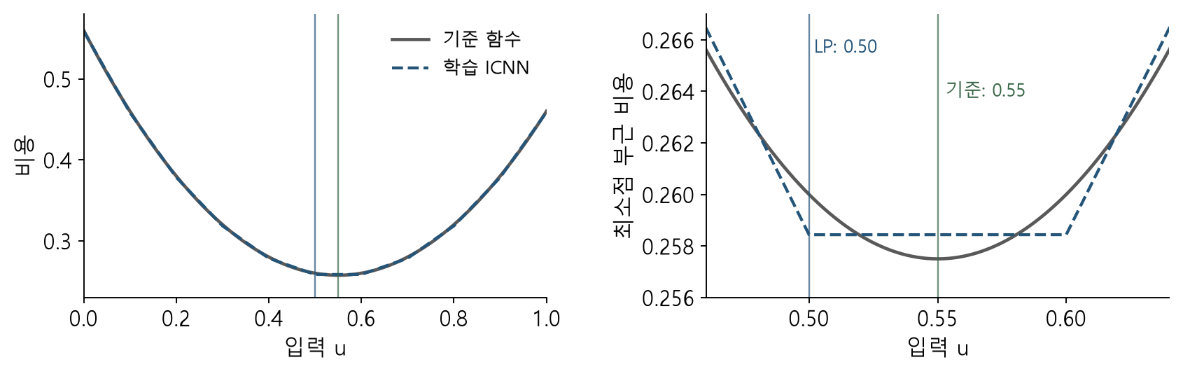
Independent-evaluation RMSE: 0.000760. LP choice: u = 0.50. Reference minimum: u = 0.55.
The reference cost difference is 0.0025. Close prediction curves can still have different minimizers.
A flat reference curve near its minimum allows a noticeable input shift with a small cost change. Input difference 0.05 and cost difference 0.0025 measure different things. Visually close prediction curves do not establish identical minimizing inputs.
Prediction error and loss from the selected input
Complete the square in q(u)=(u−0.6)²+0.1u+0.2 to obtain q(u)=(u−0.55)²+0.2575. Squared distance from the minimizer equals the cost increase.
| Input | Reference calculation | Cost |
|---|---|---|
| Reference minimum u=0.55 | 0²+0.2575 | 0.2575 |
| Model choice u=0.50 | (−0.05)²+0.2575 | 0.2600 |
| Difference | 0.2600−0.2575 | 0.0025 |
The difference 0.001563 between predicted cost 0.258437 and reference cost 0.260000 is prediction error at the selected point. Difference 0.0025 from the reference minimum is cost lost because of the selection.
These comparisons use different baselines. State the quantities subtracted in both accuracy reports and decision evaluations.
Checks on an LP result
- Save the input domain, context, scaling, and model weights.
- Check W and w signs, objective direction, and every use of outputs.
- Evaluate the original network at the chosen u and compare with the LP objective.
- Separately evaluate the reference objective and constraints.
Fitted-model LP objective: 0.258437. Reference cost: 0.260000. Difference: surrogate error.
Choosing a model structure
| Target and conditions | Approach to examine |
|---|---|
| Known convex cost minimization | ICNN or fixed-context PICNN |
| ReLU, linear output, linear outer constraints | Epigraph LP after checking its conditions |
| Concentration equalities or nonconvex response | General surrogate with an appropriate NLP/MILP |
| Weak evidence for convexity | Compare structural prediction bias and decision errors |
Running the lab and checking outputs
python -m pip install -r requirements.txt
python week07_lab.py --output-dir my-results
Extract the code bundle before running. It writes results.json, fitted coefficients, training.csv, and heldout.csv.
Automatic checks cover the hand optimum 0.16, fitted sign conditions, LP/forward agreement, the output-lower-bound counterexample, and the unbounded example. The notebook runs the same functions in stages.
Assignment: equivalence conditions and decision error
- Add a cost cap of 0.25 to the two-hinge model and calculate both endpoints of its feasible interval.
- Run the output-lower-bound counterexample and record the falsely allowed u and its true output.
- Change fitted knot spacing from 0.1 to 0.05; compare prediction error and reference decision loss.
- Explain why c is fixed and which output uses your formulation permits.
Companion: derivations and short answer checks.