Week 5: From a Predictor to an Optimization Formulation
The smallest reactor that meets product specifications
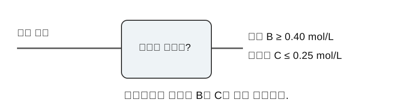
Product B must reach 0.40 mol/L while byproduct C stays below 0.25 mol/L. At fixed flow, how small can the reactor be?
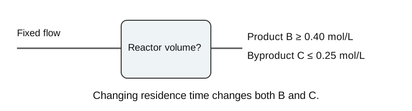
Product specifications and reactor volume minimization
Given a residence time, the network predicts outlet concentrations. Design asks for a residence time that satisfies those concentration requirements.
Longer residence converts A to B, but also converts B to C. Maximizing B and minimizing volume are different objectives.
This week: decision formulation and frozen ReLU computation using linear constraints and binary variables.
Learning objectives for optimization formulation
- Decisions, fixed context, predicted outputs, objective, and constraints
- Big-M equivalence for one ReLU: proof by branch
- Valid pre-activation bounds from the input domain
- Hand-built MILP versus forward pass at identical inputs
Submission: formulation, verification results, and solution interpretation.
Decision variables and fixed context
| Role | Value or range in the lab |
|---|---|
| Decision | Residence time τ ∈ [2, 10] min |
| Fixed context | T = 330 K, C_Af = 1.2 mol/L |
| Fixed flow | Q = 1 L/min |
| Predicted output | A, B, C concentrations y [mol/L] |
| Objective | Minimize volume V = Qτ [L] |
Here τ is a design variable selecting volume at fixed flow. Choosing temperature as well requires a model with temperature as an input and bounds over that domain.
Choosing residence time fixes the required volume through V=Qτ at fixed flow. Changing residence time in an existing vessel instead requires changing flow or another condition, which changes the variables and costs of the design problem.
An optimization problem in symbols
Notation: decisions u, fixed context d, model outputs y. Fitted weights θ: fixed.
Feasible point: satisfies network equations and process constraints. Optimum: feasible point with the smallest objective.
Prediction supplies u and computes y. Optimization treats both as unknowns and links them with y=fθ(u). Encoding that relation prevents the solver from changing y independently just to satisfy specifications.
CSTR design optimization problem
With Q = 1 L/min, minimizing τ also minimizes V. Outputs are in mol/L and must be converted to those units before checking specifications.
B ≥ 0.40 is a concentration specification. Purity or production-rate requirements need constraints written from their own definitions.
τ=2 gives a small volume but may lack sufficient B. Increasing τ until B reaches its lower bound identifies a boundary below which volume is smaller but B fails. The C upper limit must also hold at that boundary before it is a minimum feasible design.
Reference concentrations for the lab
Assume perfect mixing, constant volume, equal inlet and outlet flow, and consecutive 1:1 reactions A → B → C. At 330 K, k₁ = 0.2 min⁻¹ and k₂ = 0.1 min⁻¹.
We evaluate these equations at five residence times to construct a small ReLU model.
The frozen computational graph
ReLU: componentwise in each hidden layer. Optimization variables: inputs, intermediate values, and outputs. Numeric constants: W and b.
Making weights variable introduces products of W and h, so the MILP derived here would no longer apply.
Intermediate network values become optimization variables, but they are not free choices. Each affine equality and ReLU constraint ties one layer to the preceding layer. This converts the forward calculation into relations that must hold simultaneously.
Equality representation of input scaling
The lab maps τ to dimensionless input x. Optimization uses exactly the offset and scale used to construct the predictor.
If outputs were standardized as well, include y = μ + Ds. This inverse transformation is linear when μ and D are fixed.
For example, τ=6 gives x=(6−2)/8=0.5. Feeding 6 directly to the network leaves its 0–1 input domain. Check the coordinates entering each equation rather than relying only on variable names.
Piecewise-linear structure of ReLU
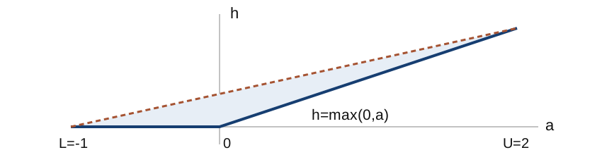
The blue line is the exact graph. The shaded region includes points admitted when the binary variable is relaxed.
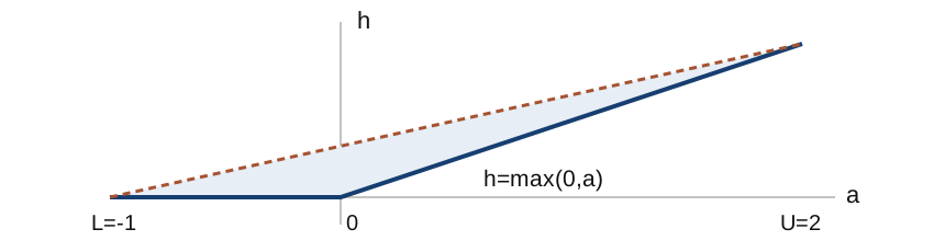
For a<0, h=0 is horizontal; for a>0, h=a is a line of slope one. Binary z selects the branch. Relaxing z to a continuous value also admits points between the branches, allowing outputs above the actual ReLU.
The ReLU graph and its lower inequalities
At a = −0.2, h = 0.4 satisfies both inequalities, although ReLU returns 0.
The objective or a later layer may favor larger h. For an arbitrary network, these lower inequalities alone are insufficient; exact graph modeling also needs branch-specific upper inequalities.
Big-M formulation of one ReLU
Assume valid finite bounds L ≤ a ≤ U with L < 0 < U.
Branches: inactive at z = 0; active at z = 1. L and U: bounds on this neuron’s pre-activation.
h≤Uz pins h to zero when z=0. h≤a−L(1−z) pins h to a when z=1. Valid L and U make the unused upper inequality permissive enough to retain every correct point on the selected branch.
Equivalence of the inactive branch (z = 0)
The remaining upper inequality, 0 ≤ a − L, holds because a ≥ L. This branch therefore represents exactly L ≤ a ≤ 0 and h = 0.
Equivalence of the active branch (z = 1)
The remaining upper inequality h ≤ U is equivalent to a ≤ U. Thus 0 ≤ a ≤ U and h = a.
At a = 0, z can be either 0 or 1, and the output h is fixed at 0.
Substituting numbers into one ReLU formulation
For a=2x−1 and x∈[0,1], L=−1,U=1. The inequalities are h≥0, h≥a, h≤a+1−z, and h≤z.
| Input and branch | Lower bound | Upper bound | Output |
|---|---|---|---|
| x=0.2, a=−0.6, z=0 | h≥0 | h≤0; h≤0.4 | h=0 |
| x=0.8, a=0.6, z=1 | h≥0.6 | h≤0.6; h≤1 | h=0.6 |
| Wrong z=0 at x=0.8 | h≥0.6 | h≤0 | Impossible |
a = 2 * x - 1
h = max(0., a)
z = int(a >= 0.)
assert h >= 0 and h >= a
assert h <= a + 1 - z and h <= z
The binary selects a branch compatible with a; it does not create an arbitrary output. At a=0, either z is possible but both give h=0.
Linear representations of stable active and inactive neurons
| Valid range | Replacement | Binary variable |
|---|---|---|
| U ≤ 0 | h = 0 | None |
| L ≥ 0 | h = a | None |
| L < 0 < U | Four Big-M inequalities | One |
Allowing inputs outside the bounded domain invalidates this simplification. Recheck bounds and classifications when changing the domain.
An interval [−2,−0.1] never activates, so replace the neuron by h=0. On [0.2,1.3], h=a everywhere. Only a possible sign change needs branch selection; bounds therefore determine which neurons require binaries.
Interval bounds accounting for weight signs
Assume lᵢ ≤ hᵢ ≤ uᵢ for every input. Negative weights reverse which input endpoint gives the minimum or maximum.
Interval arithmetic gives valid bounds, but ignoring correlations between inputs can make them wider than the attainable range.
A bound calculation by hand
The minimum occurs at (x₁, x₂) = (0, 2), and the maximum at (1, −1). Do this calculation before choosing an arbitrary large constant.
For the lower bound, use x₁=0 with positive coefficient 2 and x₂=2 with negative coefficient −3: 0−6+0.5=−5.5. Reverse those endpoints for the upper bound: 2−3×(−1)+0.5=5.5. A negative coefficient reverses the direction of an extreme.
Bound validity and formulation correctness
Using U = 0.5 at a point whose true pre-activation is a = 0.7 excludes h = 0.7: even z = 1 imposes h ≤ 0.5.
Wider valid bounds preserve the graph at integer solutions, but can weaken the continuous relaxation.
Observed extrema in the training samples do not automatically bound the entire input domain.
Frozen coefficients of the ReLU interpolant
Linearly interpolate reference concentrations at τ = 2, 4, 6, 8, 10 min. Fix the hidden hinges at those breakpoints and compute output weights from interpolation slopes.
j = 0, 1, 2, 3 and output k is A, B, or C. This lab constructs the model by interpolation rather than gradient training.
Apply the first segment slope from the start. At each later knot, an activating ReLU adds the difference between the new and old slopes. The active slope changes therefore sum to the slope of the current segment.
From interpolation slopes to ReLU weights
The first three B knot values at τ=2,4,6 are 0.285714286,0.380952381,0.409090909. Since x=(τ−2)/8, adjacent knots are 2/8=0.25 apart in x.
| Calculation | Result |
|---|---|
| First slope in x | (0.380952381−0.285714286)/0.25=0.380952381 |
| Second slope in x | (0.409090909−0.380952381)/0.25=0.112554113 |
| First ReLU weight W₀B | first slope: 0.380952381 |
| Weight W₁B at knot 0.25 | new minus previous slope: −0.268398268 |
For 0.25<x<0.5, only the first two ReLUs have derivative 1, so the total slope is 0.380952381 − 0.268398268 = 0.112554113. The new hinge is zero at its knot, preserving continuity.
Slopes computed with respect to τ must be multiplied by 8 to obtain weights for x: the same concentration change occurs over an x interval eight times shorter. Construct the A and C columns in the same way.
Neuron bounds in the lab model
| Neuron | aⱼ | Lⱼ | Uⱼ | Treatment |
|---|---|---|---|---|
| 0 | x | 0 | 1 | h₀ = x |
| 1 | x − 0.25 | −0.25 | 0.75 | Binary |
| 2 | x − 0.50 | −0.50 | 0.50 | Binary |
| 3 | x − 0.75 | −0.75 | 0.25 | Binary |
There are three binary variables. Substituting the affine pre-activations leaves eight continuous variables: one x, four h values, and three outputs.
Hidden values and B concentration at τ=5 min
Subtract thresholds [0,0.25,0.50,0.75] from x=(5−2)/8=0.375.
| j | aⱼ=x−tⱼ | hⱼ | Contribution WⱼB·hⱼ |
|---|---|---|---|
| 0 | 0.375 | 0.375 | 0.380952381×0.375=0.142857143 |
| 1 | 0.125 | 0.125 | −0.268398268×0.125=−0.033549784 |
| 2 | −0.125 | 0 | 0 |
| 3 | −0.375 | 0 | 0 |
Adding bias 0.285714286 gives B≈0.395021645 mol/L. Taking the midpoint of the 4-min and 6-min values also gives (0.380952381+0.409090909)/2=0.395021645.
The ReLU sum and segment interpolation express the same calculation. They differ from reference-process B=0.4 at 5 min, so this prediction falls slightly below the B≥0.40 specification.
Matrix representation of Big-M constraints
For neuron 1, a₁ = x − 0.25, L₁ = −0.25, and U₁ = 0.75.
Set h₁ ≥ 0 and 0 ≤ z₁ ≤ 1 as variable bounds, and declare z₁ integer. The lab assembles the full matrix in the same way.
The second row collects h₁≤x−0.25+0.25(1−z₁)=x−0.25z₁ on the left. At x=0.5,z₁=1 it gives h₁≤0.25; the first row gives h₁≥0.25, fixing h₁=0.25.
Storing one constraint as a solver row
Use variable order [x,h₀,h₁,h₂,h₃,y_A,y_B,y_C,z₁,z₂,z₃]. Only three columns are nonzero for h₁−x+0.25z₁≤0.
import numpy as np
row = [-1, 0, 1, 0, 0, 0, 0, 0, 0.25, 0, 0]
row_lower = -np.inf
row_upper = 0.0
| Substitution | Row dot product | Check |
|---|---|---|
| x=0.5,h₁=0.25,z₁=1 | −0.5+0.25+0.25=0 | satisfies upper bound 0 |
| x=0.5,h₁=0.30,z₁=1 | −0.5+0.30+0.25=0.05 | violates upper bound |
For output equality y_B−∑WⱼB hⱼ=b_B, set both row bounds to b_B. Mark the z₁ column as integer and also give it bounds [0,1]. A coefficient row alone does not make a variable binary.
SciPy LinearConstraint interprets each row as lb <= A @ v <= ub. Check variable order and coefficient signs against the same equation.
Conditions for MILP representability
A graph of fixed affine layers, ReLUs, and affine scaling can be expressed by an MILP. The objective and all remaining constraints must also be linear for the entire problem to be an MILP.
Products Qy with both flow and concentration variable, nonlinear kinetics, or sigmoid/tanh operations fall outside this formulation.
The Week 4 projection can also be appended as affine equalities when its coefficient matrices are fixed and its input dependence is affine.
MILP and forward-pass consistency at fixed inputs
Fix one residence time, remove product specifications, and solve the network equations. Compare every h and y with the forward pass.
41 checked inputs: domain endpoints, all breakpoints, both sides of interior breakpoints, and random inputs. Maximum difference: 1.25e-08.
This tests the formulation implementation. Process prediction error requires comparison with separate reference values.
Once the input is fixed, the original network output is determined. A different solver output points to weight ordering, scaling, signs, or bounds. Product specifications are separate from evaluating the network at that point, so remove them during this check.
CSTR design optimization results
| Quantity | This run |
|---|---|
| Minimum τ [min] | 5.353846 |
| Minimum V [L] | 5.353846 |
| Predicted [A, B, C] [mol/L] | [0.584615, 0.400000, 0.215385] |
| Binary [z₁, z₂, z₃] | [1, 0, 0] |
| Termination | optimal, status = 0 |
The B lower bound is active, while the C upper bound has slack. Independent segmentwise linear calculations give the same residence time.
B slack is 0.400000−0.40=0; C slack is 0.25−0.215385=0.034615 mol/L. A small decrease in τ makes B insufficient first. This active constraint prevents a further volume reduction.
Interpolation fraction at the product lower bound
Across 4–6 min, B increases from 0.380952381 to 0.409090909. Divide the required increase by the full segment increase.
| Calculation | Value |
|---|---|
| Required B increase | 0.40−0.380952381=0.019047619 |
| Full segment increase | 0.409090909−0.380952381=0.028138528 |
| Segment fraction α | 0.019047619/0.028138528≈0.676923077 |
| Residence time | 4+2α≈5.353846154 min |
| C at the same α | 0.152380952+α(0.245454545−0.152380952)≈0.215384615 |
B is below 0.40 on all earlier segments. At this first crossing, C≤0.25 and nonnegativity also hold, giving the minimum volume. Comparing interpolated B with C at a different τ would not check specifications for the same design.
Formulation equivalence and process prediction error
The MILP exactly represents the frozen interpolant. This property does not remove its process approximation error.
At the selected τ = 5.353846 min, the reference concentrations are [0.579495, 0.404137, 0.216369] mol/L, which differ from the predictor.
The solution is optimal for the specified surrogate problem. A process design decision also requires checking reference-process specifications and comparing objective values.
LP relaxation and objective lower bounds
Relaxing z to [0, 1] gives a lower bound on the MILP optimum for minimization. Intermediate values and outputs may nevertheless leave the network graph.
With L = −1, U = 2, a = 0, the relaxed point z = 1/3, h = 2/3 is feasible, although the ReLU output is 0.
The LP and MILP objective values coincide in this CSTR example. Equality of objectives in one instance does not establish general graph equivalence.
Enlarging a minimization feasible set retains the original optimum, so the new optimal value cannot be larger. This makes the LP value a lower bound. Its outputs may leave the network graph, so an LP solution is not automatically an acceptable design.
Run the lab and prepare the submission
python -m pip install -r requirements.txt
python week05_lab.py --output-dir my-results
- Hand checks: one neuron’s bounds and matrix signs
- Checks in
results.json: forward error and termination status - Translate one row of
milp_matrix.csvback into an equation. - Change the B lower bound from 0.40 to 0.41 and explain whether feasibility remains.
Sources and assigned reading
Boyd & Vandenberghe, Convex Optimization, §4.1: variables, objectives, and feasible sets.
Anderson et al., Strong mixed-integer programming formulations for trained neural networks, §2.1: the ReLU Big-M formulation.
SciPy milp documentation: bounds, integrality, LinearConstraint, and return status.