Week 4: Learning with Physical Constraints
Mismatch between predicted total and feed concentration
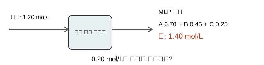
An MLP predicts [0.70, 0.45, 0.25] mol/L for A, B, and C with a 1.20 mol/L feed. The total is 1.40. Can an engineer pass this outlet to the next process unit?
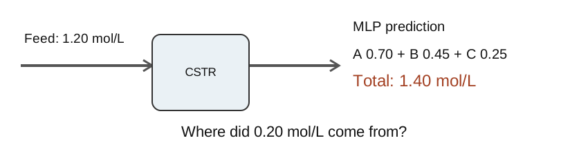
Propagation of balance errors between process units
The next separator calculates its load from incoming component amounts. A total-concentration error in the reactor surrogate enters that calculation directly, so prediction error and balance violation need separate checks.
This week: residual penalties in the loss, output projection onto specified linear equalities, and component errors before and after correction.
Comparisons for learning with physical constraints
- MLP, soft sum penalty, and hard sum projection on the same data
- Nearest-point projection from KKT conditions; rank assumptions
- Hand gradients versus automatic differentiation through a fixed layer
- Separate reporting: component errors, equality violations, negative concentrations, and unenforced balances
Lab reference: the Week 2 steady-state CSTR.
Reference process and units
Assume perfect mixing, constant volume, and equal inlet/outlet flow. The feed contains only A; consecutive reactions A → B → C have 1:1 stoichiometry. Temperature T is prescribed and the model has no energy balance.
At 330 K, k₁ = 0.2 min⁻¹ and k₂ = 0.1 min⁻¹. With τ = 5 min and C_Af = 1.2 mol/L, [C_A, C_B, C_C] = [0.6, 0.4, 0.2] mol/L.
Steady-state balances and the concentration-sum equality
Let r_A, r_B, and r_C denote the right sides of the steady-state species balances. Adding them cancels the reaction terms.
At steady state each residual is zero, giving S = C_A + C_B + C_C = C_Af. This concentration-sum equality depends on the stated stoichiometry and flow assumptions. Other reactions require the appropriate elemental or mass balance and units.
Each amount converted from A to B appears once negatively in A and once positively in B. Conversion from B to C cancels in the same way. Only external inflow and outflow remain in the sum balance; this cancellation justifies the total-concentration constraint.
Componentwise prediction error and concentration-sum error
| Prediction [mol/L] | Component error [mol/L] | Sum residual [mol/L] |
|---|---|---|
| [0.70, 0.45, 0.25] | [+0.10, +0.05, +0.05] | +0.20 |
| [0.70, 0.30, 0.20] | [+0.10, −0.10, 0.00] | 0.00 |
The reference is [0.60, 0.40, 0.20] mol/L. The second prediction has the right sum but incorrect A and B. An equality-only evaluation would miss those errors.
Definition of physical residuals
The sum residual is r_sum = C_A + C_B + C_C − C_Af, in mol/L. Known kinetics also allow species-level steady-state residuals.
Units for these three residuals: mol/(L·min). Training: sum residual only. Separate evaluation: species residuals.
For [0.7,0.3,0.2] at 330 K and τ=5, species residuals are [−0.04,0.05,−0.01] mol/(L·min). They sum to zero although individual steady balances fail. One sum constraint does not replace three species equations.
Data-error and constraint-violation terms in a soft penalty
Both terms are dimensionless with = 1 mol/L. The lab uses λ = 10; its meaning includes the averaging conventions for one sum residual and three component errors.
Changing λ changes the objective and gradient magnitudes. A finite penalty and a completed training run do not guarantee zero residual at every input.
One gradient moves predictions toward data; another moves the sum toward the constraint. When those directions conflict, a finite λ can produce a compromise. Compare the averaging conventions of both terms, not only the numerical λ.
Solve a finite-penalty problem by hand
Minimize the scalar objective ½(z − a)² + ½λ(z − b)², where data favor a, the equality requires z = b, and λ ≥ 0. Setting the derivative to zero gives:
If a ≠ b, a residual remains for finite λ. Very large penalties also require attention to loss magnitudes and numerical conditioning.
Collecting the derivative terms gives (1+λ)z=a+λb. With a=1.4,b=1.2,λ=9, this is 10z=12.2, hence z=1.22. The data derivative −0.18 cancels the penalty derivative 9×0.02=+0.18, although the equality residual remains 0.02.
Differentiation targets in automatic differentiation
Our MLP maps [T, τ, C_Af] to steady concentrations. Training differentiates the loss with respect to parameters θ. The sum residual and steady-state species balances need no time derivative.
A continuous-time PINN using y_θ(t) may have a residual ∂y_θ/∂t − F(y_θ, u), which also differentiates with respect to a coordinate. Distinguish this from the parameter gradient used for training.
If t̃ = (t − μ_t)/s_t, then ∂y/∂t = (1/s_t)∂y/∂t̃.
Hard linear equalities and feasible output sets
x ∈ ℝᵖ, y ∈ ℝⁿ, A ∈ ℝᵐˣᵖ, B ∈ ℝᵐˣⁿ, and b ∈ ℝᵐ. Coefficients A, B, b are fixed; the raw output is ŷ = f_θ(x).
For the CSTR, x = [T, τ, C_Af], A = [0, 0, −1], B = [1, 1, 1], and b = 0. Thus d(x) = C_Af.
Fixing x also fixes d(x). The sum constraint fixes one combination of three outputs rather than all three values. It leaves freedom to exchange A and B while preserving the sum.
Nearest-point projection onto a linear equality set
Fixed quantities: x and raw prediction ŷ. Adjusted variable: output z. Metric: Euclidean distance in physical concentration coordinates.
The objective is strictly convex, so a nonempty feasible set has a unique projected output. KKT conditions give a closed form for this equality-only QP.
The aim is to satisfy the sum while disturbing a nearby prediction as little as possible. Equal units and weights lead to minimizing the squared correction norm. Protecting selected components more strongly requires an explicitly weighted distance.
Lagrangian and KKT conditions
Enforce stationarity and primal feasibility together.
There are no inequalities, hence no complementary slackness or multiplier sign restriction. For a strictly convex objective with affine equalities, an output satisfying these conditions is the global minimizer.
Stationarity says that the correction lies along the constraint normals Bᵀ. Motion tangent to the equality set does not repair the residual but increases distance, so it is absent from the nearest-point correction.
Eliminate the multiplier to obtain the projection
Stationarity gives z = ŷ − Bᵀλ. Substitute into Bz = d.
If rank(B) = m, then G = BBᵀ is positive definite. The formula uses an inverse for notation; implementation solves Gλ = Bŷ − d. A fixed B allows reuse of a factorization or fixed projection coefficients.
There are m multiplier unknowns, one per equality. Compute the original residual Bŷ−d, solve the system with G, then multiply by Bᵀ to turn constraint-space coefficients into a correction across n outputs.
The fixed affine output layer in KKT-hPINN
Physical equalities determine this layer’s coefficients; they are not trained. MLP weights θ are trained using the projected output in the loss.
The specified equalities hold during training and inference, subject in implementation to floating-point error and linear-system conditioning. Source: Chen et al. (2024).
Constraint-matrix rank and equality-system consistency
| Case | Consequence |
|---|---|
| rank(B) = m ≤ n | Every d is attainable; BBᵀ is invertible. |
| Redundant rows, consistent d | Feasible outputs exist but BBᵀ is singular. Use independent rows or an SVD. |
| Redundant rows, inconsistent d | No feasible output exists. A pseudoinverse cannot satisfy all equations. |
For nearly dependent rows, inspect rank tolerance and conditioning. Scaling entire equality rows consistently changes numerical scales without changing the feasible set.
Project the concentration sum by hand
Subtract the same 0.066667 mol/L from each component. The total is 1.20, but the output still differs from the reference [0.60, 0.40, 0.20].
Displayed values are rounded. Keep full precision during calculation and check the final sum residual.
From the sum residual to projected output
The raw output is [0.70,0.45,0.25] and the target total is 1.20 mol/L. Equal corrections Δ give 1.40−3Δ=1.20, hence Δ=0.20/3.
| Step | Value |
|---|---|
| Bŷ−d | 1.40−1.20=0.20 |
| G=BBᵀ | 1²+1²+1²=3 |
| Solve Gλ=residual | λ=0.0666667 |
| Component corrections | [−0.0666667,−0.0666667,−0.0666667] |
| Projected output | [0.6333333,0.3833333,0.1833333] |
Equal correction has squared distance 3×(0.20/3)²=0.013333. Subtracting 0.20 only from A also repairs the sum but has squared distance 0.04. This explains equal correction under an equally weighted Euclidean metric.
Projecting onto two independent equalities
Consider a linear example requiring both total concentration 1.2 and A−B=0.2. The rows of constraint matrix B are [1,1,1] and [1,−1,0], with right side [1.2,0.2]. Project raw output [0.70,0.45,0.25].
| Step | Calculation |
|---|---|
| Residuals Bŷ−d | [0.20,0.05] |
| Diagonal entries of G=BBᵀ | row squared norms: 3 and 2 |
| Off-diagonal entry | 1×1+1×(−1)+1×0=0 |
| Solve Gλ=residual | λ=[0.20/3,0.05/2] |
| Bᵀλ | [0.091667,0.041667,0.066667] |
| Projected output | [0.608333,0.408333,0.183333] |
The sum is 1.2 and A−B=0.2. Independence allows the two residuals to be removed separately. If the second row were twice the first, G would have no inverse.
Here B names the constraint matrix, distinct from product species B. The additional A−B equality is a condition of this linear calculation example.
Post-projection and training through projection
| Method | Output used in the training loss |
|---|---|
| MLP + post-projection | Train on raw outputs; project at test time. |
| KKT-hPINN approach | Use projected outputs throughout training. |
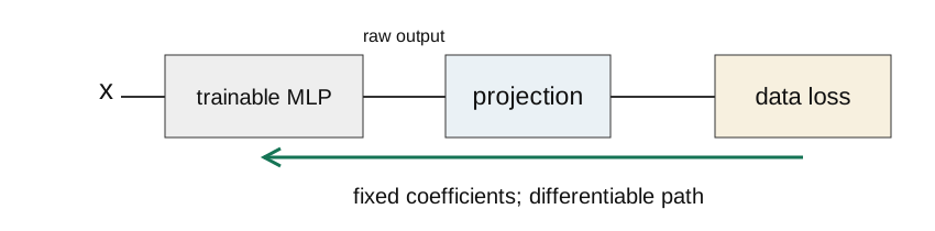
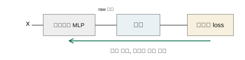
Both can satisfy the same equality, but their training gradients differ and generally produce different parameters.
Post-projection repairs the sum after training. During projected training, loss sees the corrected output. Directions that projection removes, such as adding the same amount to every raw component under a sum constraint, contribute no gradient from that output loss.
Backpropagation through a fixed projection layer
P is a symmetric orthogonal projector, so Pᵀ = P. The projection matrix P is fixed and passes the output gradient to the raw prediction by multiplying it by Pᵀ.
Detaching the output or wrapping projection in no_grad cuts the required path. The parameter gradient continues through the MLP Jacobian by the chain rule.
Check the backward pass with three components
An upstream gradient [1, 0, 0] at the projected output becomes [2/3, −1/3, −1/3] at the raw output. Its sum is zero, so it lies in the equality’s tangent space.
Additional checks: analytic Jacobian and double-precision gradcheck for two independent equalities.
The mean of gradient [1,0,0] is 1/3. Subtracting it gives [2/3,−1/3,−1/3]. Raising all components equally changes the sum and is removed; directions that redistribute concentration while preserving the sum remain.
Constraint-matrix transformation under output standardization
Compute μ and positive scales s_j from training data only. A projection in standardized coordinates z must use BD and right side d − Bμ.
Projection in standardized coordinates minimizes a distance in physical coordinates that weights each squared component correction by 1/s_j². Specify the correction metric and scales.
Projection metric and component corrections
Minimizing distance in standardized coordinates with scales [0.2,0.5,0.1] allocates physical corrections in proportion to squared scales. Split the residual 0.20 in the ratio 0.04:0.25:0.01.
| Component | Squared-scale fraction | Subtracted concentration | Result |
|---|---|---|---|
| A | 0.04/0.30 | 0.026667 | 0.673333 |
| B | 0.25/0.30 | 0.166667 | 0.283333 |
| C | 0.01/0.30 | 0.006667 | 0.243333 |
scales = np.array([0.2, 0.5, 0.1])
raw = np.array([0.70, 0.45, 0.25])
weights = scales**2 / np.sum(scales**2)
projected = raw - (raw.sum() - 1.2) * weights
B has the largest scale, making a physical correction less costly in standardized distance. It therefore changes more. Checking only the final sum 1.20 hides the difference between these metrics.
Let Δⱼ be the correction. Minimize ½∑Δⱼ²/sⱼ² subject to ∑Δⱼ=−0.20. Stationarity gives Δⱼ/sⱼ²+λ=0, hence Δⱼ=−λsⱼ². Substituting into the sum constraint gives λ=0.20/∑sⱼ², which explains the squared-scale proportions.
Physical-unit restoration and projection order
The MLP returns standardized outputs z. Restore mol/L with μ + Dz, then project in physical coordinates. Divide data errors by the common scale = 1 mol/L.
D is diagonal, hence Dᵀ = D. A loss divided by component-specific standard deviations adds weights that must also enter gradient and error interpretations.
A minimal PyTorch implementation
raw units: mol/L. feed shape: (batch, 1).
raw = y_mean + y_scale * net(x_scaled)
residual = raw.sum(dim=-1, keepdim=True) - feed
y_projected = raw - residual / 3.0
loss = ((y_projected - y_true) / c_scale).square().mean()
optimizer.zero_grad()
loss.backward()
optimizer.step()
Projection adds no trainable parameters.
keepdim=True retains residual shape (batch,1), broadcasting the same correction across the three components of each row. Summing the whole batch into one number would incorrectly share corrections across operating conditions.
Concentration-sum constraints and nonnegativity
Raw [0.02, 0.90, 0.50] mol/L sums to 1.42. Projection to 1.20 gives [−0.053333, 0.826667, 0.426667] mol/L.
The sum is correct and A is negative. Clamping just the negative value to zero changes the sum to about 1.253333.
To require both nonnegativity and the sum, use a method including those inequalities, such as simplex projection. Its gradient changes by region as active inequalities change.
Recomputing projection with nonnegativity
Subtracting the sum residual 0.22 equally from [0.02,0.90,0.50] makes A negative. Requiring both the sum and nonnegativity leads to recomputation on the boundary A=0.
| Step | Calculation |
|---|---|
| Fix A at zero | B+C=1.20 |
| Remaining raw sum | 0.90+0.50=1.40 |
| Correction to each free component | (1.40−1.20)/2=0.10 |
| Result | [0,0.80,0.40] mol/L |
Subtract 0.10 from each positive component while A stops at zero. This is the simplex projection of the raw output. Clipping only the negative entry does not readjust B and C, so it does not restore the sum.
As raw values change, the active constraint changes when A becomes positive again. The derivative is therefore not one fixed matrix over the entire domain, unlike fixed linear-equality projection.
Conditions for error reduction by projection
If reference lies in the same affine set, orthogonality gives:
Thus physical-space projection of the same raw prediction cannot increase total squared Euclidean error. An individual component error can increase.
If noisy labels lie outside the set, or projection uses another weighted metric, this physical Euclidean comparison does not directly apply. The identity also does not rank two separately trained models.
Raw error separates into a normal component violating the sum and a tangent component distributing concentrations incorrectly. Projection removes only the normal part. Orthogonality makes their squared norms add, so total squared error cannot increase for the same feasible reference and metric.
Fix the comparison protocol
Use T = 305-355 K, τ = 1-8 min, C_Af = 0.8-1.5 mol/L. Rates are k₁ = 0.2 exp[6000(1/330 − 1/T)] and k₂ = 0.1 exp[5000(1/330 − 1/T)] min⁻¹.
Train/validation/test have 900/300/300 rows, seed 404, and noise-free analytic labels. All models are 3 → 32 → 32 → 3 ReLU MLPs with 1283 parameters.
They share initial weights, batch order, and training statistics. Use Adam 0.001, batches of 128, and the minimum validation physical MSE among 600 epochs; then evaluate test.
Run results: accuracy and equality violations
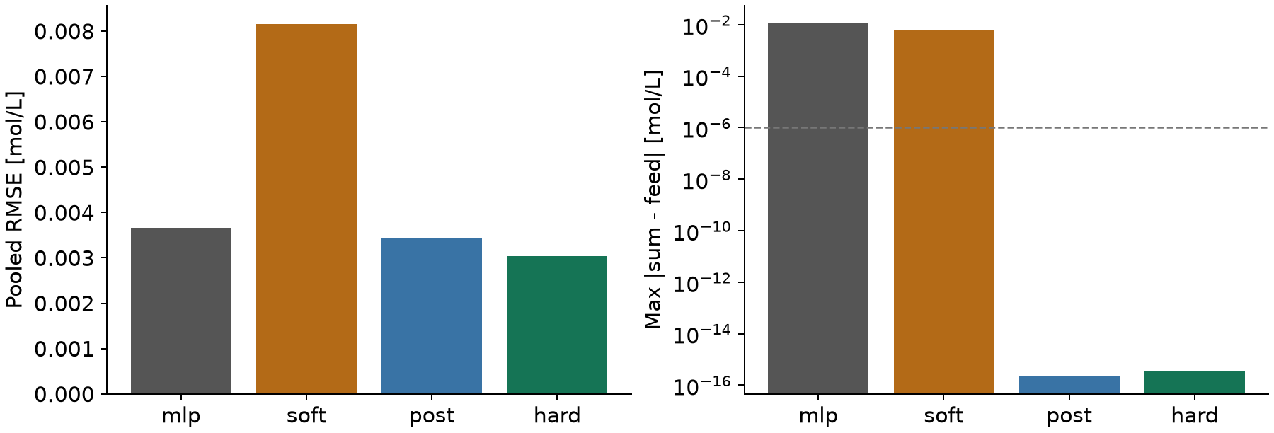
| Model | Pooled RMSE | Max sum violation | Negative entries |
|---|---|---|---|
| MLP | 0.003657 | 1.17e-02 | 1 |
| Soft (λ = 10) | 0.008161 | 6.30e-03 | 5 |
| MLP + post | 0.003426 | 2.22e-16 | 1 |
| Hard | 0.003036 | 3.33e-16 | 1 |
Concentration and error units: mol/L. Negative-entry count: values below −10⁻⁸ among 900 test component values.
In this run, the soft penalty reduced sum violations but increased RMSE. Hard and post satisfied the sum while retaining negative concentrations. One seed does not establish a general accuracy ranking.
Component RMSE and minimum concentration
| Model | A RMSE | B RMSE | C RMSE | Minimum |
|---|---|---|---|---|
| MLP | 0.003866 | 0.003383 | 0.003704 | -0.003451 |
| Soft (λ = 10) | 0.008753 | 0.008742 | 0.006840 | -0.010393 |
| MLP + post | 0.003724 | 0.003015 | 0.003500 | -0.004176 |
| Hard | 0.003728 | 0.002540 | 0.002703 | -0.002822 |
All quantities are in mol/L. Pooled RMSE can hide differences between components.
The minimum covers every component and test row. Record the evaluation tolerance and the actual minimum together.
Evaluation of species balances omitted from training
The hard model satisfies the concentration-sum equality, while its component reaction/outlet relations retain a residual RMS of 0.002225 mol/(L·min).
Zero sum residual corresponds to the species residuals summing to zero. Positive and negative species residuals can cancel, leaving nonzero species RMS. The figure tests these additional relations that were not enforced in training.
Run the lab and retain the evidence
Download the lab ZIP, notebook, or Python script. Extract the ZIP and run in that folder.
python -m pip install -r requirements.txt
python week04_lab.py --check-only
python week04_lab.py --output-dir week04-results
Outputs retain the split dataset, test predictions, weights, training statistics, validation history, and evaluation JSON. The supplied run used CPU, float64, and PyTorch 2.14.1+cpu.
Total-concentration equality in the dynamic model
With constant feed and τ within an interval, the exact total-concentration transition is:
If S_k differs from C_Af, do not immediately force the next total to C_Af. B = [1, 1, 1] still acts on the next state, but the right side is the transition above.
When τ is an input, the equality right side d(x) depends nonlinearly on τ. Compute that right side, then apply the projection with fixed B.
Exercises and submission
- Project [0.70, 0.45, 0.25] onto total 1.20; backpropagate an upstream gradient [1, 0, 0].
- Explain feasibility for B rows [1, 1, 1], [2, 2, 2] and d = [1.2, 2.5].
- Compare λ = 0.1, 1, 10 using validation; evaluate only the selected setting on test.
- Submission for each model: A/B/C RMSE, sum MAE/max, minimum concentration, and species-balance residuals
Next week: frozen ReLU predictor and optimization-problem definition.
Reading companion and papers
Week 4 companion · English reading PDF
Chen, H., Constante Flores, G. E., & Li, C. (2024). Physics-informed neural networks with hard linear equality constraints. Computers & Chemical Engineering, 189, 108764. DOI · Public manuscript · Author code/data.
Raissi, M., Perdikaris, P., & Karniadakis, G. E. (2019). Physics-informed neural networks: A deep learning framework for solving forward and inverse problems involving nonlinear partial differential equations. Journal of Computational Physics, 378, 686-707. DOI.
Mathematics and implementation sources
Boyd, S., & Vandenberghe, L. (2004). Convex Optimization. Section 5.5.3 on KKT conditions and Section 10.1 on equality-constrained minimization. Official book.
Official PyTorch documentation: linear solves, numerical gradient checks. Raissi et al., 2017 Part I manuscript.