Week 3: Predicting Dynamic Responses and Rollout
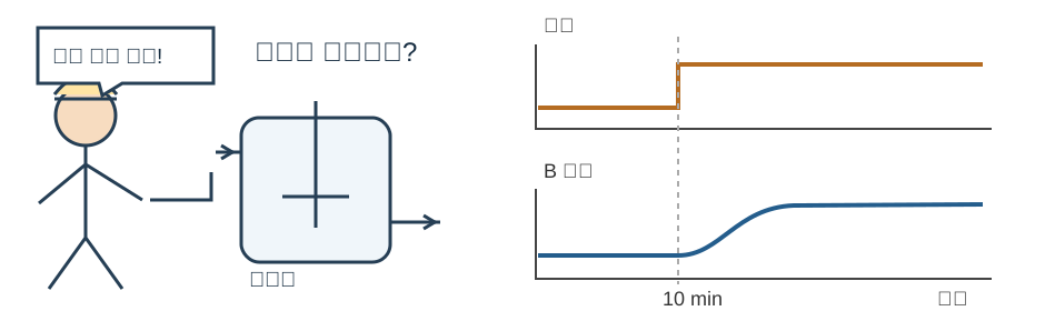
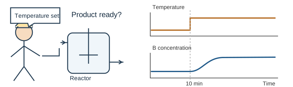
The temperature changed. Is the product ready?
A process engineer changes a reactor’s temperature at 10 min. A product tank receives its outlet immediately. How will B concentration change over the next 20 min?
The journey to a new steady state matters
During a grade change or startup, material produced before the target composition is reached can require separation or reprocessing. The endpoint alone does not describe that transient.
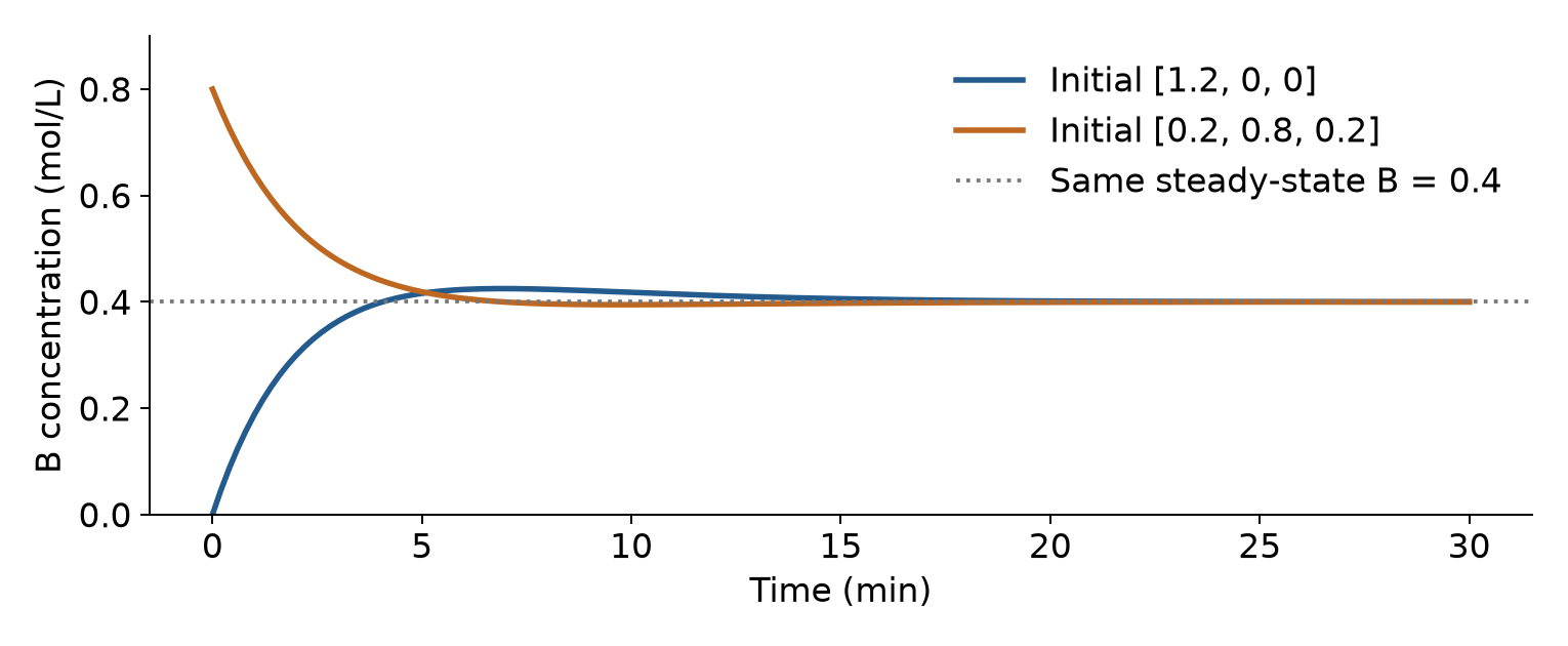
The same temperature can give different current compositions. The contents already inside the tank affect the next response. We will learn a short state transition and reuse it to predict the entire trajectory.
What we will build
- Define the current state, prescribed future inputs, fixed context, and sampling interval.
- Train a state-transition MLP on concentration increments.
- Compare one-step predictions and 30 min rollout on held-out trajectories.
Submit the same model’s component errors in both evaluations, error versus horizon, and two temperature-plan trajectories. RNN/LSTM and encoder–decoder are optional extensions.
A steady-state map becomes a transition map
Week 2: [T, τ, C_Af] → the composition after equilibration.
Week 3: current composition + interval input + context → composition one interval later.
Repeatedly applying this map produces a trajectory. A feedforward MLP can model a dynamic transition when its inputs contain the state needed for that transition.
State, future input, and fixed context
| Quantity | Meaning | Unit / role |
|---|---|---|
| c_k = [C_A,k, C_B,k, C_C,k] | Current reactor composition | mol/L; state |
| u_k = T_k | Temperature over interval k | K; prescribed input |
| q = [τ, C_Af] | Residence time and feed concentration | min, mol/L; fixed per trajectory |
| Δt = 0.2 | Sampling interval | min; fixed for this model |
Specify c_0 and the complete temperature sequence before rollout. The temperature plan is supplied by the exercise.
The reference CSTR
An ideal, perfectly mixed reactor has constant volume and equal inlet/outlet flow. Its consecutive first-order reactions are A → B → C with 1:1 stoichiometry. Feed contains A only. Temperature is prescribed; an energy balance is not included.
k₁(T) = 0.2 exp[6000(1/330 − 1/T)], k₂(T) = 0.1 exp[5000(1/330 − 1/T)] in min⁻¹. At 330 K, k₁ = 0.2 and k₂ = 0.1 min⁻¹.
A continuous process, sampled at fixed times
For each interval [t_k, t_k + Δt), hold T_k constant. Integrate the balances over that interval to obtain c_k+1. The state stays continuous when the input switches.
30 min / 0.2 min = 150 transitions, with 151 sampled states. The temperature step at 10 min starts at interval index 50.
The learned map predicts a 0.2 min transition. Increasing the number of applications extends the horizon; it does not change the sampling interval.
An exact interval response for this teaching model
With constant interval inputs, the balances are affine in the state. Write dc/dt = Mc + b. The steady state c∗ satisfies Mc∗ + b = 0.
The lab evaluates this expression analytically. It generates labels at the selected Δt. The reading companion derives M and the component formulas.
At c₀ = [1.2, 0, 0], T = 330 K, τ = 5 min, feed = 1.2 mol/L: c₁ ≈ [1.153870, 0.045672, 0.000458] mol/L.
Build trajectories before building transition rows
Use 300–360 K, τ = 1–10 min, and feed = 0.8–1.5 mol/L. Random temperature plans contain six 5 min blocks. Each trajectory has its own initial composition, with nonnegative components summing to feed.
| Split | Trajectories | Transition rows |
|---|---|---|
| Train | 60 | 9000 |
| Validation | 15 | 2250 |
| Test | 20 | 3000 |
What does one training row contain?
| Fields | Construction |
|---|---|
| Input v_k | [C_A,k, C_B,k, C_C,k, T_k, τ, C_Af] |
| Next-state label | c_k+1 from the reference interval response |
| Increment target | Δc_k = c_k+1 − c_k |
| Identification | split, trajectory ID, t_k |
The target is a change in mol/L.
The transition MLP and its scaling
Use 6 → 32 → 32 → 3, ReLU hidden layers, and a linear output. The parameter count is (6×32 + 32) + (32×32 + 32) + (32×3 + 3) = 1379.
Compute input and increment means/standard deviations from train rows. Apply those same statistics to validation, test, and rollout states.
The MLP predicts standardized increments. Restore each increment to mol/L before adding it to the current state. An increment model can represent a zero change, but its architecture alone does not guarantee accuracy or physical consistency.
Train on reference current states
Each train input contains the reference current state. Minimize the mean squared standardized increment error.
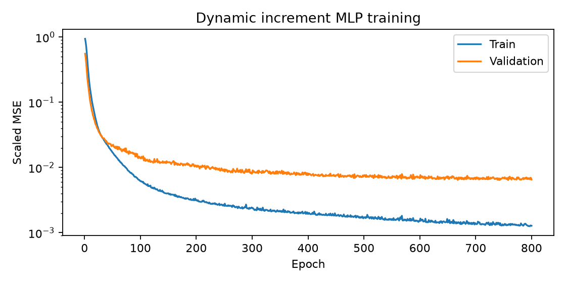
Adam: learning rate 0.001, batch size 512, up to 800 epochs. Retain the weights with minimum validation loss. Test trajectories are used after this selection.
Training history
Two ways to evaluate the same model
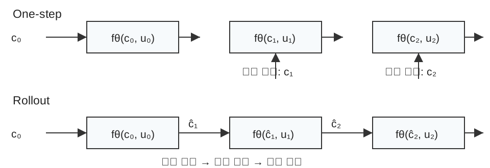
One-step: reset the input to the reference state at every time.
Rollout: start at c₀, then feed each predicted state into the next transition. Keep all future inputs and the context identical in both evaluations.
The one-step result uses more state information than a forecast started only once.
Where the next state comes from
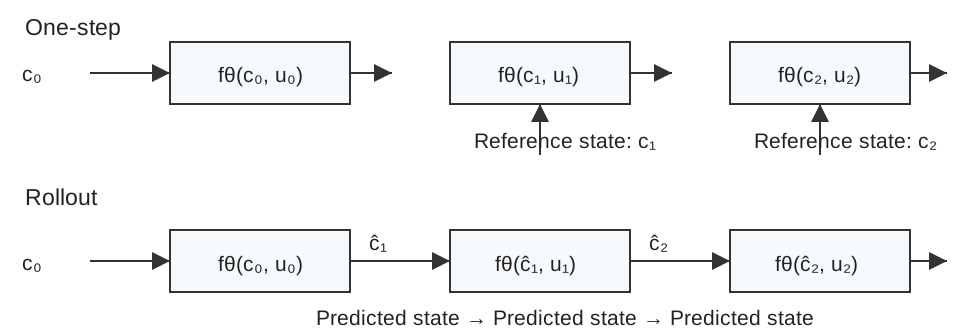
Both diagrams use the same frozen transition model.
A rollout is a short, explicit loop
Given an initial state and 150 future input intervals:
pred = np.empty((len(controls) + 1, 3))
pred[0] = initial_state
for k, control in enumerate(controls):
    pred[k + 1] = dynamic_step(
        model, scaling, pred[k:k+1], control[None, :]
    )[0]
No reference state enters this loop after initialization. Evaluate all 150 predicted states.
How local error propagates
Let e_k = ĉ_k − c_k. Add and subtract the prediction at the reference state:
The first difference transports the existing state error through the learned map. δ_k is the local prediction error at the reference state. Even a small δ_k enters each successive prediction.
Small one-step error can accumulate
For a scalar illustration, let the reference be F(c) = 0.9c and the learned map be f(c) = 0.9c + 0.001. Start with e₀ = 0.
One-step bias is 0.001; at 10 recursive steps the error is about 0.00651. A contracting map limits the accumulation. A different state sensitivity can produce a different horizon pattern.
The state sensitivity matters too
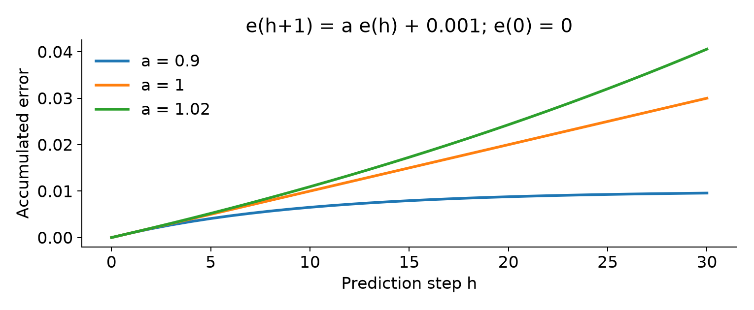
These are scalar examples, not fitted CSTR results. Actual rollout errors can increase, level off, or change sign.
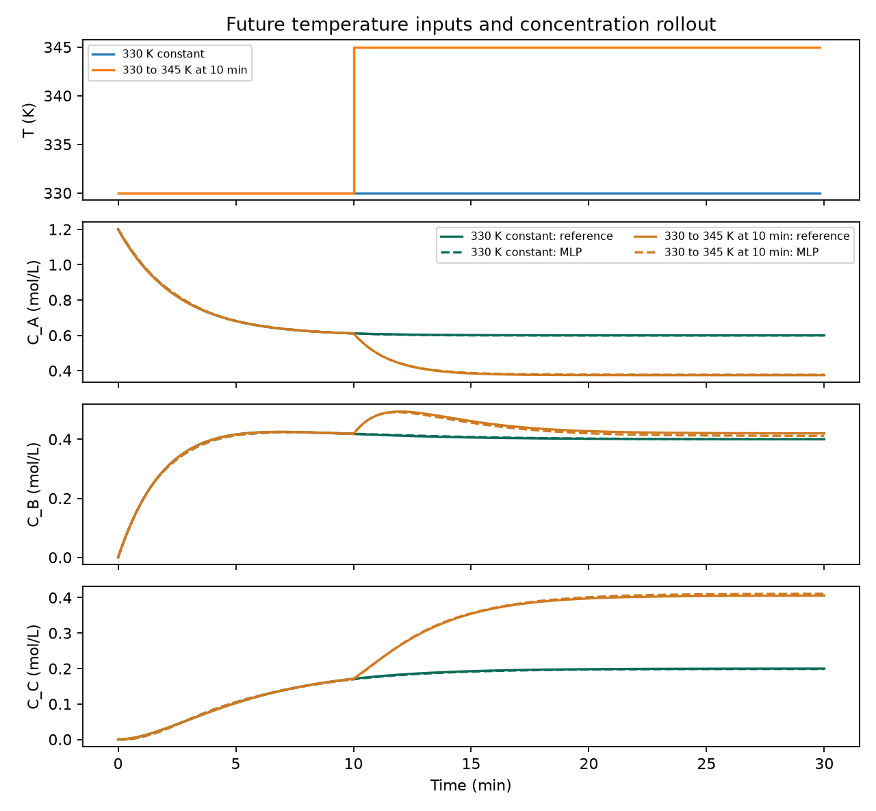
Two prescribed temperature plans
| Setting | Constant plan | Step plan |
|---|---|---|
| Initial composition, mol/L | [1.2, 0, 0] | [1.2, 0, 0] |
| τ; C_Af | 5 min; 1.2 mol/L | 5 min; 1.2 mol/L |
| 0 ≤ t < 10 min | 330 K | 330 K |
| 10 ≤ t ≤ 30 min | 330 K | 345 K |
Compare reference trajectories and the MLP rollout under exactly the same plans. Check when the curves separate and how they approach their new steady response.
A, B, and C over the full trajectory
Compare error in physical units
| RMSE, mol/L | A | B | C |
|---|---|---|---|
| One-step | 0.001170 | 0.001288 | 0.001163 |
| Rollout | 0.009465 | 0.009629 | 0.010425 |
Results from 20 held-out trajectories, 150 predicted times each. Rollout errors are larger in this stored run. Compute per-component RMSE across the 3000 predictions, then also inspect each horizon separately.
Here n indexes test trajectories, h the number of transitions, and j the component.
Read the error versus horizon
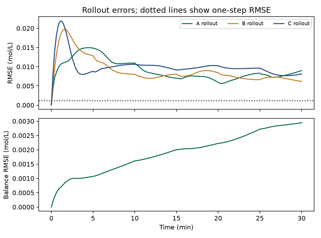
Physical checks along the trajectory
With S₀ = C_Af and fixed feed, the reference sum stays equal to feed. The learned outputs need not satisfy this relation.
| Check, mol/L | One-step | Rollout |
|---|---|---|
| Sum-residual RMSE | 0.000051 | 0.002014 |
| Minimum prediction | -0.001152 | -0.005166 |
Return to the engineer’s question
| B at 30 min, mol/L | Reference | MLP rollout |
|---|---|---|
| Constant 330 K | 0.400091 | 0.399819 |
| 330 → 345 K at 10 min | 0.420021 | 0.411526 |
Both calculations give more B at 30 min under the step plan. The MLP underestimates the step-plan endpoint by about 0.00850 mol/L. Its trajectory shows the transient that an endpoint steady-state prediction would miss.
A time-dependent product specification would require checking the relevant interval, not just this final sample.
Run the local lab and submit the comparison
The supplied lab bundle includes the reference, stored model, scaling, plots, and notebook.
python -m pip install -r requirements.txt
python week03_lab.py --output-dir week03-results
# Optional: train again with the same data construction
python week03_lab.py --train --output-dir week03-retrained
Submit state/input definitions, split/scaling details, one-step and rollout RMSE, horizon plots, and the two temperature-plan trajectories.
Exercises and direct reading
- Derive dS/dt and state the condition for S to remain equal to feed.
- Compute the first 0.2 min transition and compare it with forward Euler.
- Explain why the same MLP receives different state inputs in the two evaluations.
- Change an initial state while keeping the input plan fixed. Compare both reference and predicted trajectories.
The reading companion provides derivations, worked numbers, code, and answer checks. It develops the local-error recurrence and an optional multi-step training objective.
Optional: when a hidden state helps
The core example supplies all three concentration states and prescribed temperature. If measurements omit relevant states, a history of observations and inputs can help reconstruct them.
An RNN updates a learned hidden state. An LSTM adds gated memory updates. Compare these models with the same trajectory split and forecast information.
Optional: an encoder and a trajectory decoder
Encoder: summarize past observations and inputs into a state representation.
Decoder: predict the future concentration sequence using that representation and the prescribed future input plan. Ensure each future input reaches the corresponding prediction step.
Read Sutskever, Vinyals & Le (2014), Sections 1–2, for the sequence-to-sequence idea.
Original paper · Further derivations are in the supplied reading.